
Time series analysis of armed robberies in Boston
Data: Monthly armed robberies
Techniques: ARIMA models, stationarity tests, differencing
This project looks at monthly Boston armed robberies from Jan 1966-Oct 1975. Here I build a quick ARIMA model to forecast robberies.
Data originally from : McCleary & Hay (1980)
%matplotlib inline
import sys
import pandas as pd
import numpy as np
from datetime import datetime
from statsmodels.tsa.stattools import adfuller
from statsmodels.tsa.seasonal import seasonal_decompose
from statsmodels.tsa.stattools import acf, pacf
from statsmodels.tsa.arima_model import ARIMA

import matplotlib.pylab as plt
from matplotlib.pylab import rcParams
rcParams['figure.figsize'] = 15, 6

print('Python version: %s.%s.%s' % sys.version_info[:3])
print('numpy version:', np.__version__)
print('pandas version:', pd.__version__)
Python version: 3.5.2
numpy version: 1.11.1
pandas version: 0.18.1
def check_stationarity(timeseries):

    # Determine rolling statistics (moving averages and variance)
    rolmean = pd.rolling_mean(timeseries, window=12)
    rolstd = pd.rolling_std(timeseries, window=12)

    # Plot rolling statistics:
    orig = plt.plot(timeseries, color='blue',label='Original')
    mean = plt.plot(rolmean, color='red', label='Rolling Mean')
    std = plt.plot(rolstd, color='black', label = 'Rolling Std')
    plt.legend(loc='best')
    plt.title('Rolling Mean & Standard Deviation')
    plt.show(block=False)

    # Perform Dickey-Fuller test:
    print('Results of Dickey-Fuller Test:')
    dftest = adfuller(timeseries, autolag='AIC')
    dfoutput = pd.Series(dftest[0:4], index=['Test Statistic','p-value','#Lags Used','Number of Observations Used'])
    for key,value in dftest[4].items():
        dfoutput['Critical Value (%s)'%key] = value
    print(dfoutput)
The data
data = pd.read_csv('monthly-boston-armed-robberies-j.csv',parse_dates=True, index_col='Month')
data.head()
data.dtypes
Monthly Boston armed robberies    int64
dtype: object
# To confirm that dtype=datetime, or that it is a datetime object
data.index
DatetimeIndex(['1966-01-01', '1966-02-01', '1966-03-01', '1966-04-01',
               '1966-05-01', '1966-06-01', '1966-07-01', '1966-08-01',
               '1966-09-01', '1966-10-01',
               ...
               '1975-01-01', '1975-02-01', '1975-03-01', '1975-04-01',
               '1975-05-01', '1975-06-01', '1975-07-01', '1975-08-01',
               '1975-09-01', '1975-10-01'],
              dtype='datetime64[ns]', name='Month', length=118, freq=None)
# Converting to a series object for convenience
ts = data['Monthly Boston armed robberies']
ts.head()
Month
1966-01-01    41
1966-02-01    39
1966-03-01    50
1966-04-01    40
1966-05-01    43
Name: Monthly Boston armed robberies, dtype: int64
Check stationarity
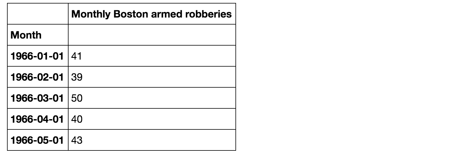
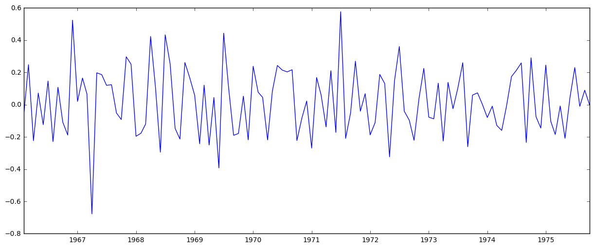
plt.plot(ts)
It’s clear that there’s an overall increasing trend, and the time series is clearly not stationary, but let’s look at the moving averages/variance and implement the Dickey-Fuller test for stationarity:
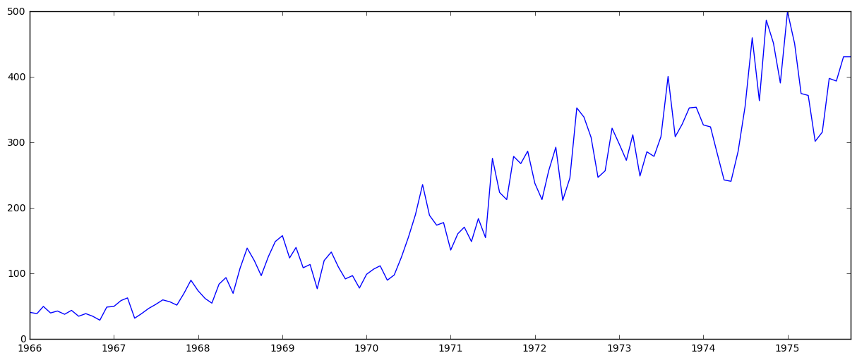
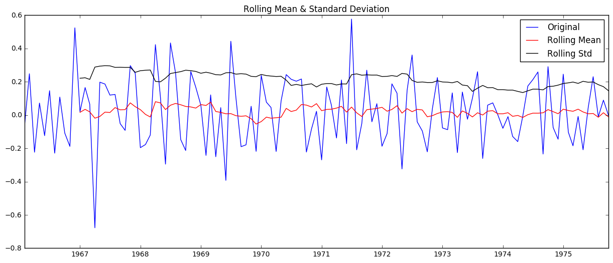
check_stationarity(ts)
Results of Dickey-Fuller Test:
Test Statistic                   1.001102
p-value                          0.994278
#Lags Used                      11.000000
Number of Observations Used    106.000000
Critical Value (1%)             -3.493602
Critical Value (10%)            -2.581533
Critical Value (5%)             -2.889217
dtype: float64
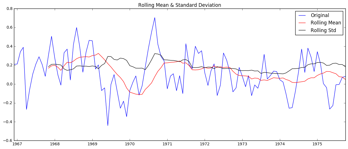
The mean (in red) is clearly increasing with time and the test statistic is much larger than the critical values, so we can’t reject the null hypothesis- aka this is not a stationary series.
Make the series stationary
Eliminating trend
In this case there is a significant positive trend. Let’s first work on estimating and eliminating it. We can do a simple log transform (which would penalize higher values more than smaller ones).
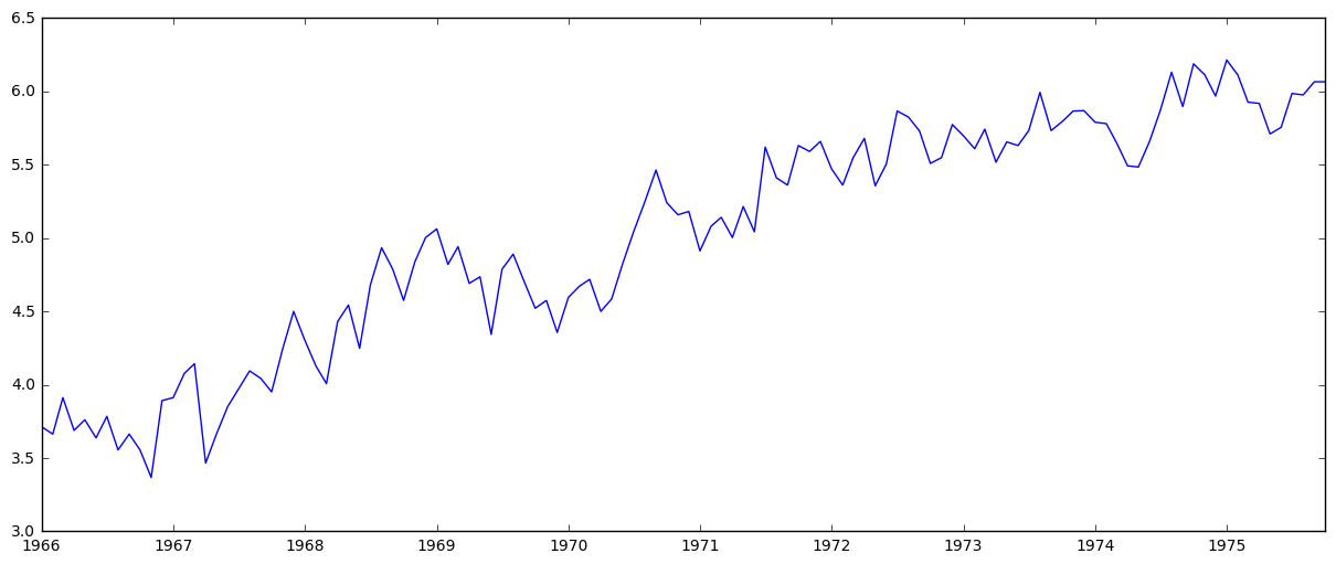
ts_log = np.log(ts)
plt.plot(ts_log)
As well as smoothing by taking rolling averages:
moving_avg = pd.rolling_mean(ts_log,12)
plt.plot(ts_log)
plt.plot(moving_avg, color='red')
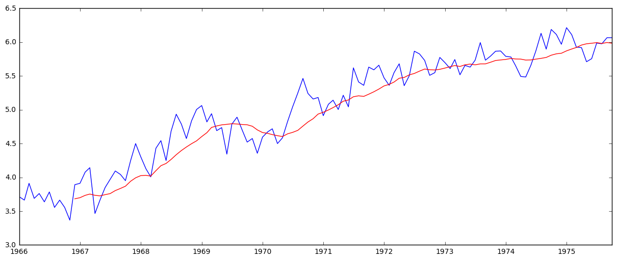
The red shows the rolling average. Now subtract it from the original series.
Note: since we are taking the mean of the last 12 values, rolling mean is not defined for the first 11 values:
# Subtract rolling average
ts_log_moving_avg_diff = ts_log - moving_avg
ts_log_moving_avg_diff.head(12)
Month
1966-01-01         NaN
1966-02-01         NaN
1966-03-01         NaN
1966-04-01         NaN
1966-05-01         NaN
1966-06-01         NaN
1966-07-01         NaN
1966-08-01         NaN
1966-09-01         NaN
1966-10-01         NaN
1966-11-01         NaN
1966-12-01    0.208955
Name: Monthly Boston armed robberies, dtype: float64
So the first 11 are Nan. Let’s drop these and then check for stationarity again:
ts_log_moving_avg_diff.dropna(inplace=True)
check_stationarity(ts_log_moving_avg_diff)
Results of Dickey-Fuller Test:
Test Statistic                  -5.323692
p-value                          0.000005
#Lags Used                       0.000000
Number of Observations Used    106.000000
Critical Value (1%)             -3.493602
Critical Value (10%)            -2.581533
Critical Value (5%)             -2.889217
dtype: float64
Now we get a test statistic that is smaller than the 1% critical value.
Now let’s try a weighted moving average (where more recent values get higher weight)- more specifically an exponentially weighted moving average, where weights are assigned to all the previous values with a decay factor:
expwighted_avg = pd.ewma(ts_log, halflife=12)
plt.plot(ts_log)
plt.plot(expwighted_avg, color='red')
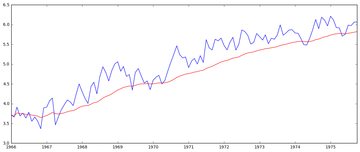
Now we remove this from the series and check for stationarity:
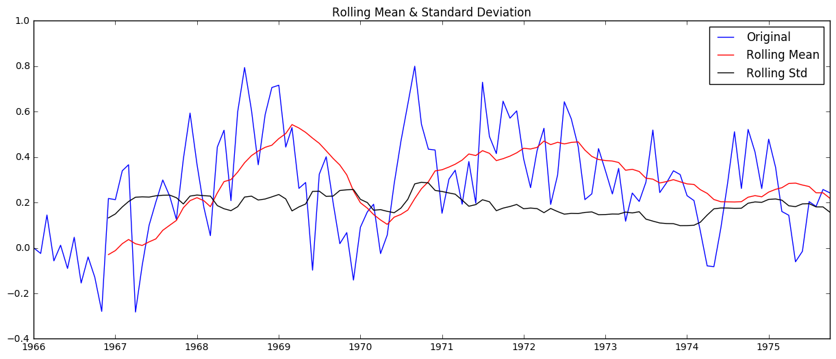
ts_log_ewma_diff = ts_log - expwighted_avg
check_stationarity(ts_log_ewma_diff)
Results of Dickey-Fuller Test:
Test Statistic                  -5.155717
p-value                          0.000011
#Lags Used                       0.000000
Number of Observations Used    117.000000
Critical Value (1%)             -3.487517
Critical Value (10%)            -2.580124
Critical Value (5%)             -2.886578
dtype: float64
This actually isn’t better than the previous method of using the simple moving average.
Removing trend and seasonality with differencing
Now let’s try another method of removing trend, as well as seasonality: differencing.
ts_log_diff = ts_log - ts_log.shift()
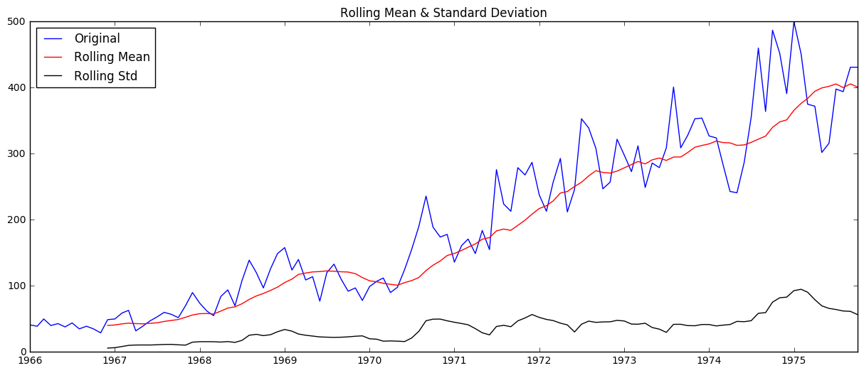
plt.plot(ts_log_diff)
The trend looks like it’s gone.
Check stationarity:
ts_log_diff.dropna(inplace=True)
check_stationarity(ts_log_diff)
Results of Dickey-Fuller Test:
Test Statistic                -7.601792e+00
p-value                        2.378602e-11
#Lags Used                     3.000000e+00
Number of Observations Used    1.130000e+02
Critical Value (1%)           -3.489590e+00
Critical Value (10%)          -2.580604e+00
Critical Value (5%)           -2.887477e+00
dtype: float64
Again, the test statistic is significantly lower than the 1% critical value so this time series is very close to stationary.
Forecasting
For ARIMA we need the parameters p, d, and q. Here d is the number of nonseasonal differences. We use these plots to determine p and q:
# ACF (autocorrelation function) and PACF (partial autocorrelation function) plots:
lag_acf = acf(ts_log_diff, nlags=20)
lag_pacf = pacf(ts_log_diff, nlags=20, method='ols')

# Plot ACF:
plt.subplot(121)
plt.plot(lag_acf)
plt.axhline(y=0,linestyle='--',color='gray')
plt.axhline(y=-1.96/np.sqrt(len(ts_log_diff)),linestyle='--',color='gray')
plt.axhline(y=1.96/np.sqrt(len(ts_log_diff)),linestyle='--',color='gray')
plt.title('Autocorrelation Function')

# Plot PACF:
plt.subplot(122)
plt.plot(lag_pacf)
plt.axhline(y=0,linestyle='--',color='gray')
plt.axhline(y=-1.96/np.sqrt(len(ts_log_diff)),linestyle='--',color='gray')
plt.axhline(y=1.96/np.sqrt(len(ts_log_diff)),linestyle='--',color='gray')
plt.title('Partial Autocorrelation Function')
plt.tight_layout()
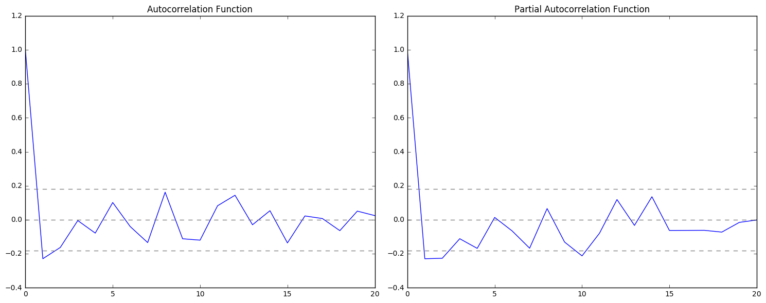
The two dotted lines on either sides of 0 are confidence intervals. These can be used to determine ‘p’ and ‘q’ values as (p: the lag value where the PACF chart crosses the upper confidence interval for the first time, q: the lag value where the ACF chart crosses the upper confidence interval for the first time).
It looks like p is roughly 1 and q is roughly equal to 1. For now I will use these values to build a model and come back to refining later.
ARIMA
For now I’ll justtry 3 different ARIMA models considering individual as well as combined effects.
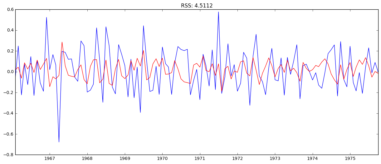
# AR (auto-regression) model
model = ARIMA(ts_log, order=(1, 1, 0))  # (p,d,q)
results_AR = model.fit(disp=-1)
plt.plot(ts_log_diff)
plt.plot(results_AR.fittedvalues, color='red')

# Print the RSS- values for the residuals
plt.title('RSS: %.4f'% sum((results_AR.fittedvalues-ts_log_diff)**2))
# MA (moving avg) model
model = ARIMA(ts_log, order=(0, 1, 1))
results_MA = model.fit(disp=-1)
plt.plot(ts_log_diff)
plt.plot(results_MA.fittedvalues, color='red')
plt.title('RSS: %.4f'% sum((results_MA.fittedvalues-ts_log_diff)**2))
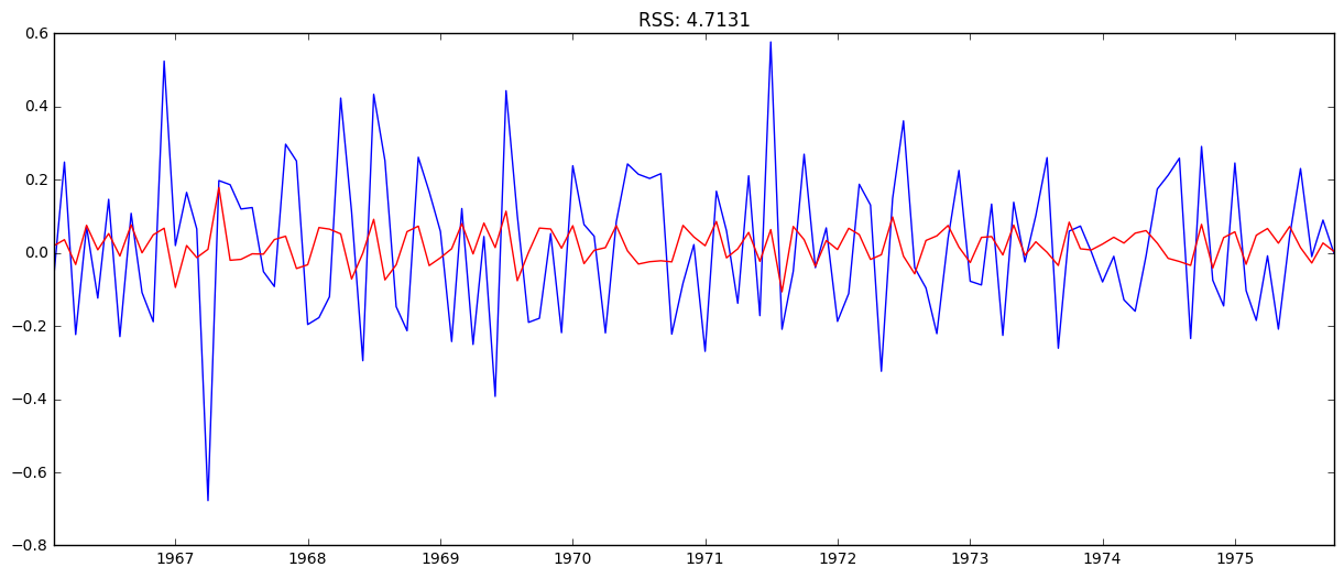
# Combined model
model = ARIMA(ts_log, order=(1, 1, 1))
results_ARIMA = model.fit(disp=-1)
plt.plot(ts_log_diff)
plt.plot(results_ARIMA.fittedvalues, color='red')
plt.title('RSS: %.4f'% sum((results_ARIMA.fittedvalues-ts_log_diff)**2))
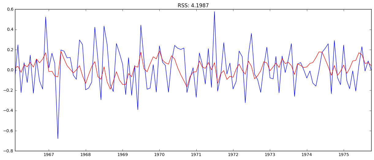
The combined gave the lowest RSS.
Next we take these values back to the original scale:
Back to the original scale
Scaling back to the original values:
predictions_ARIMA_diff = pd.Series(results_ARIMA.fittedvalues, copy=True)
print(predictions_ARIMA_diff.head())
Month
1966-02-01    0.021240
1966-03-01    0.036438
1966-04-01   -0.023285
1966-05-01    0.051275
1966-06-01    0.031915
dtype: float64
Convert differencing to log scale by adding these difference consecutively to the base number. One way to do that is to first determine the cumulative sum at index, then add it to the base number. Cumulative sum:
predictions_ARIMA_diff_cumsum = predictions_ARIMA_diff.cumsum()
print(predictions_ARIMA_diff_cumsum.head())
Month
1966-02-01    0.021240
1966-03-01    0.057678
1966-04-01    0.034392
1966-05-01    0.085667
1966-06-01    0.117582
dtype: float64
Next we add them to the base number, First create a series with all values as base number and add differences to it:
predictions_ARIMA_log = pd.Series(ts_log.ix[0], index=ts_log.index)
predictions_ARIMA_log = predictions_ARIMA_log.add(predictions_ARIMA_diff_cumsum,fill_value=0)
predictions_ARIMA_log.head()
Month
1966-01-01    3.713572
1966-02-01    3.734812
1966-03-01    3.771250
1966-04-01    3.747964
1966-05-01    3.799239
dtype: float64
Then take the exponent and compare with the original series.
predictions_ARIMA = np.exp(predictions_ARIMA_log)
plt.plot(ts)
plt.plot(predictions_ARIMA)
plt.title('RMSE: %.4f'% np.sqrt(sum((predictions_ARIMA-ts)**2)/len(ts)))
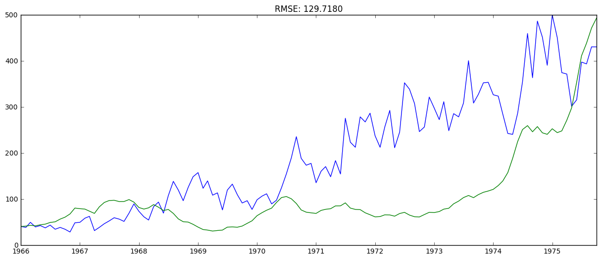
And that’s the forecast at the original scale. It’s not great; this was just a quick and dirty forecast, but after this, I’ll come back and refine the model by:
- Using seasonal ARIMA, for which I would need to find (p,d,q,P,D,Q) values.
- Get a holdout sample (validatiaon set) using recent past data points.
- Run through different parameter values and get the values that give the lowest error on the validation set.