Predicting churn from user attributes
Data: Telecom customer data
Techniques: Calculating churn probability and expected loss, random forest
Here I look at a telecom customer data set. Each row contains customer attributes such as call minutes during different times of the day, charges incurred for services, duration of account, and whether or not the customer left or not.
import pandas as pd
import numpy as np
from sklearn.preprocessing import StandardScaler
from sklearn.model_selection import train_test_split
from sklearn.cross_validation import KFold
from sklearn.grid_search import GridSearchCV
from sklearn.svm import SVC
from sklearn.ensemble import RandomForestClassifier as RF
from sklearn.linear_model import LogisticRegression as LR
from sklearn.metrics import confusion_matrix

import matplotlib.pyplot as plt
from ggplot import *
%matplotlib inline
Functions for selecting or evaluating models or returning probabilties:
class EstimatorSelectionHelper:

    """
    A helper class for running parameter grid search across different models.
    It takes two dictionaries. The first contains the models to be scored.
    The second contains the parameters for each model
    """

    def __init__(self, models, params):
        if not set(models.keys()).issubset(set(params.keys())):
            missing_params = list(set(models.keys()) - set(params.keys()))
            raise ValueError("Some estimators are missing parameters: %s" % missing_params)
        self.models = models
        self.params = params
        self.keys = models.keys()
        self.grid_searches = {}

    """
    fit(X,y) method runs a parameter grid search with cross validation for each model
    and for the given training data. If scoring=None, the score method of the estimator is used.
    """

    def fit(self, X, y, cv=3, n_jobs=1, verbose=1, scoring=None, refit=False):
        for key in self.keys:
            print("Running GridSearchCV for %s." % key)
            model = self.models[key]
            params = self.params[key]
            gs = GridSearchCV(model, params, cv=cv, n_jobs=n_jobs,
                              verbose=verbose, scoring=scoring, refit=refit)
            gs.fit(X,y)
            self.grid_searches[key] = gs

    """
    After calling fit(X,y), the score_summary() method returns a df with a summary of the scores
    """

    def score_summary(self, sort_by='mean_score'):
        def row(key, scores, params):
            d = {
                 'estimator': key,
                 'min_score': min(scores),
                 'max_score': max(scores),
                 'mean_score': np.mean(scores),
                 'std_score': np.std(scores),
                }

            return pd.Series(dict(list( params.items()) + list(d.items() ))) #sum up two dicts

        rows = [row(k, gsc.cv_validation_scores, gsc.parameters)
                for k in self.keys
                for gsc in self.grid_searches[k].grid_scores_]
        df = pd.concat(rows, axis=1).T.sort([sort_by], ascending=False)

        columns = ['estimator', 'min_score', 'mean_score', 'max_score', 'std_score']
        columns = columns + [c for c in df.columns if c not in columns]

        return df[columns]

def run_prob_cv(X, y, clf_class, **kwargs):
    """
    Returns probability of label
    """
    kf = KFold(len(y), n_folds=5, shuffle=True)
    y_prob = np.zeros((len(y),2))
    for train_index, test_index in kf:
        X_train, X_test = X[train_index], X[test_index]
        y_train = y[train_index]
        clf = clf_class(**kwargs)
        clf.fit(X_train, y_train)
        # Predict probabilities, not classes
        y_prob[test_index] = clf.predict_proba(X_test)
    return y_prob

def run_cv(X,y,clf_class,**kwargs):
    # Construct a kfolds object
    kf = KFold(len(y),n_folds=5,shuffle=True)
    y_pred = y.copy()

    # Iterate through folds
    for train_index, test_index in kf:
        X_train, X_test = X[train_index], X[test_index]
        y_train = y[train_index]
        # Initialize a classifier with key word arguments
        clf = clf_class(**kwargs)
        clf.fit(X_train,y_train)
        y_pred[test_index] = clf.predict(X_test)
    return y_pred
Functions for calibration and discrimination:
# This code from ericchiang
def calibration(prob,outcome,n_bins=10):
    """Calibration measurement for a set of predictions.
    When predicting events at a given probability, how far is frequency
    of positive outcomes from that probability?
    NOTE: Lower scores are better
    prob: array_like, float
        Probability estimates for a set of events
    outcome: array_like, bool
        If event predicted occurred
    n_bins: int
        Number of judgement categories to prefrom calculation over.
        Prediction are binned based on probability, since "descrete"
        probabilities aren't required.
    """
    prob = np.array(prob)
    outcome = np.array(outcome)

    c = 0.0
    # Construct bins
    judgement_bins = np.arange(n_bins + 1) / n_bins
    # Which bin is each prediction in?
    bin_num = np.digitize(prob,judgement_bins)
    for j_bin in np.unique(bin_num):
        # Is event in bin
        in_bin = bin_num == j_bin
        # Predicted probability taken as average of preds in bin
        predicted_prob = np.mean(prob[in_bin])
        # How often did events in this bin actually happen?
        true_bin_prob = np.mean(outcome[in_bin])
        # Squared distance between predicted and true times num of obs
        c += np.sum(in_bin) * ((predicted_prob - true_bin_prob) ** 2)
    return c / len(prob)

def discrimination(prob,outcome,n_bins=10):
    """Discrimination measurement for a set of predictions.
    For each judgement category, how far from the base probability
    is the true frequency of that bin?
    NOTE: High scores are better
    prob: array_like, float
        Probability estimates for a set of events
    outcome: array_like, bool
        If event predicted occurred
    n_bins: int
        Number of judgement categories to prefrom calculation over.
        Prediction are binned based on probability, since "descrete"
        probabilities aren't required.
    """
    prob = np.array(prob)
    outcome = np.array(outcome)

    d = 0.0
    # Base frequency of outcomes
    base_prob = np.mean(outcome)
    # Construct bins
    judgement_bins = np.arange(n_bins + 1) / n_bins
    # Which bin is each prediction in?
    bin_num = np.digitize(prob,judgement_bins)
    for j_bin in np.unique(bin_num):
        in_bin = bin_num == j_bin
        true_bin_prob = np.mean(outcome[in_bin])
        # Squared distance between true and base times num of obs
        d += np.sum(in_bin) * ((true_bin_prob - base_prob) ** 2)
    return d / len(prob)

def print_measurements(pred_prob):
    """
    Print calibration error and discrimination
    """
    churn_prob, is_churn = pred_prob[:,1], y == 1
    print("  %-20s %.4f" % ("Calibration Error", calibration(churn_prob, is_churn)))
    print("  %-20s %.4f" % ("Discrimination", discrimination(churn_prob,is_churn)))
    print("Note -- Lower calibration is better, higher discrimination is better")
Function that ties everything together and calculates expected loss from churn:
def ChurnModel(df, X, y, model):
    """
    Calculates probability of churn and expected loss,
    and gathers customer's contact info
    """
    # Collect customer meta data
    response = df[['Area Code','Phone']]
    charges = ['Day Charge','Eve Charge','Night Charge','Intl Charge']
    response['customer_worth'] = df[charges].sum(axis=1)

    # Make prediction
    clf = model()
    clf = clf.fit(X,y)
    churn_prob = clf.predict_proba(X)
    response['churn_prob'] = churn_prob[:,1]

    # Calculate expected loss
    response['expected_loss'] = response['churn_prob'] * response['customer_worth']
    response = response.sort('expected_loss', ascending=False)

    # Return response DataFrame
    return response
The data
df = pd.read_csv('churn.csv')
col_names = df.columns.tolist()
col_names
['International Plan',
 'Mail Plan',
 'Mail Message',
 'Day Minutes',
 'Day Calls',
 'Day Charge',
 'Evening Minutes',
 'Evening Calls',
 'Eve Charge',
 'Night Mins',
 'Night Calls',
 'Night Charge',
 'International Minutes',
 'International Calls',
 'Intl Charge',
 'CustServ Calls',
 'State',
 'Area Code',
 'Phone',
 'Account Length',
 'Churn?']
df.head()
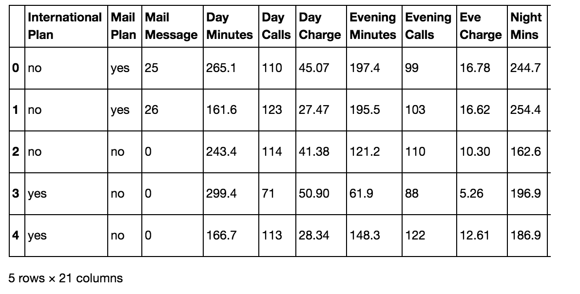
Preprocessing
The target label here is ‘Churned’ (Yes or No)
# Get the target
churn = df['Churn?']
# Convert to 0 or 1
y = np.where(churn == 'True.',1,0)

# Dropping columns we don't need
to_drop = ['Area Code', 'Phone', 'State','Churn?']
features = df.drop(to_drop, axis=1)

# Convert yes/no to Booleans
yes_no_cols = ["International Plan","Mail Plan"]
features[yes_no_cols] = features[yes_no_cols] == 'yes'

# Get updated list of feature names
feature_names = features.columns

# Prep and scale
X = features.as_matrix().astype(np.float)
scaler = StandardScaler()
X = scaler.fit_transform(X)
X.shape
(3333, 17)
Some basic models.
I won’t look for optimal parameters for now.
# Models to try
models = {
    'LR': LR(),
    'RF': RF(),
    'SVM': SVC()
}

# Paramaters to try (empty for now)
params = {
    'LR':{},
    'RF':{},
    'SVM':{}
}

X_train, X_test, y_train, y_test = \
        train_test_split(X, y, test_size=0.3, random_state = 0)

helper = EstimatorSelectionHelper(models, params)
helper.fit(X_train, y_train, n_jobs=-1)
helper.score_summary()
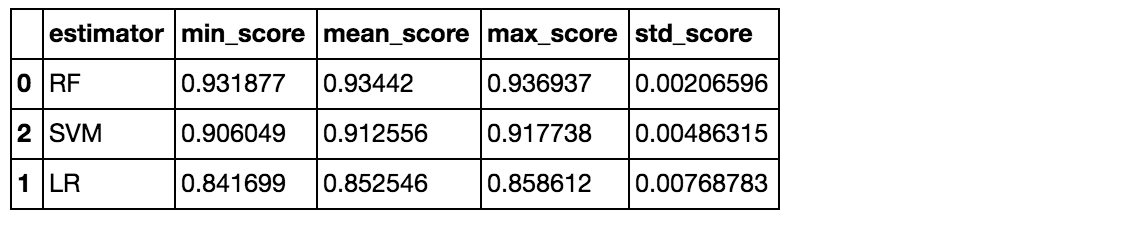
Random forest seemed to be best.
Get probability of churning
We might want to know the probability someone will churn in order to make decisions, like who to reach out to first.
# Use 10 estimators so predictions are all multiples of 0.1
pred_prob = run_prob_cv(X, y, RF, n_estimators=10)
pred_churn = pred_prob[:,1]
is_churn = y == 1
# Number of times a predicted probability is assigned to an observation
counts = pd.value_counts(pred_churn)

# Calculate true probabilities
true_prob = {}
for prob in counts.index:
    true_prob[prob] = np.mean(is_churn[pred_churn == prob])
    true_prob = pd.Series(true_prob)

# Add to dataframe
counts = pd.concat([counts,true_prob], axis=1).reset_index()
counts.columns = ['pred_prob', 'count', 'true_prob']
counts
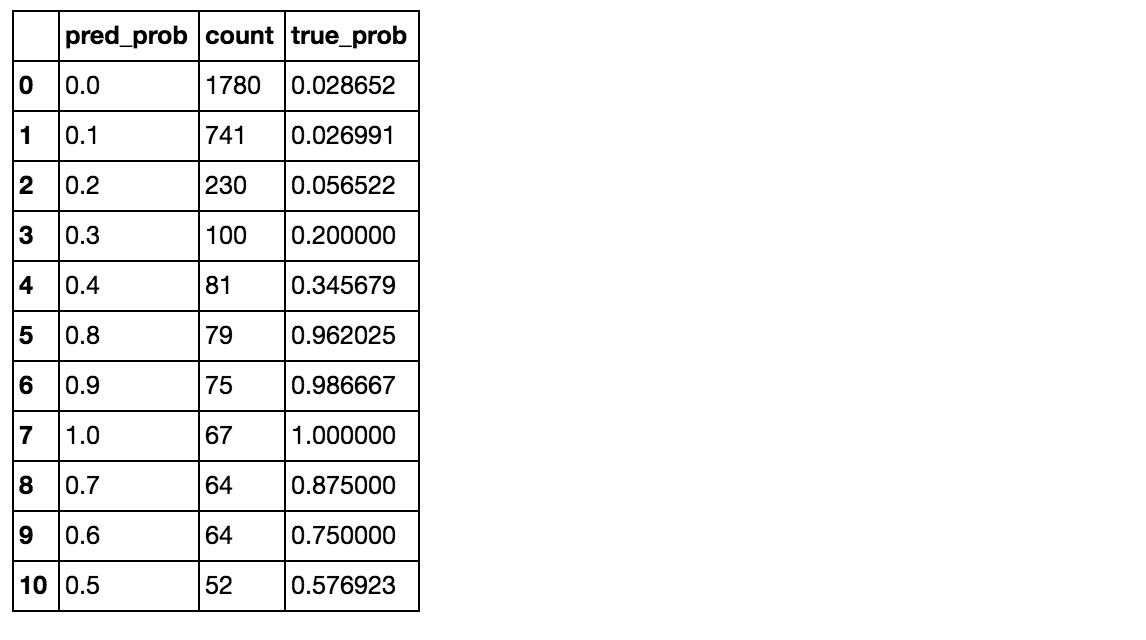
The random forest model predicted (for example) that 75 people had a 0.9 probability of churning and in actuality that group had about a .987 rate.
Calibration and discrimination
Calibration is a measure of how close predictions are to perfect predictions for a given group. Discrimination measures how far the predictions are from the baseline probability of churning.
print("Support vector machines:")
print_measurements(run_prob_cv(X,y,SVC,probability=True))

print("Random forests:")
print_measurements(run_prob_cv(X,y,RF,n_estimators=18))

print("Logistic regression:")
print_measurements(run_prob_cv(X,y,LR))
Support vector machines:
  Calibration Error    0.0004
  Discrimination       0.0655
Random forests:
  Calibration Error    0.0063
  Discrimination       0.0847
Logistic regression:
  Calibration Error    0.0016
  Discrimination       0.0257
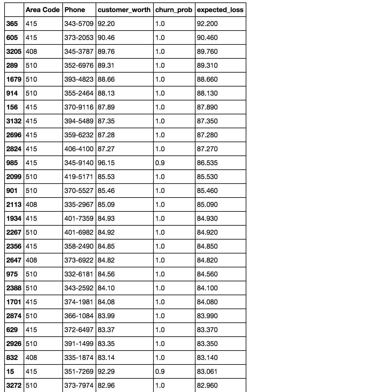
Expected loss
Finally, we calculate the expected loss by churn, sort by expected loss, and gather customer contact info.
ChurnModel(df, X, y, RF)