
Recommending wines and segmenting wine drinkers
Data: Wine sales data
Techniques: k-means clustering, recommender systems, matrix factorization
Part I- Clustering Wine Drinkers
Part II- Recommending Wines
Part 1- Segmenting wine drinkers
Here I explore online sales data for a wine store based in the Upper East Side in NYC. Although online sales are not representative of total sales for this particular store (most of their sales are in-store), it will be informative to take a look at what online customers are buying.
In Part 2 I’ll use this data to build wine recommenders.
%matplotlib inline

import pandas as pd
import numpy as np
from sklearn.cluster import KMeans
from sklearn.decomposition import PCA
from sklearn import metrics
from ggplot import *
import matplotlib.pyplot as plt
import seaborn as sns
data = pd.read_csv('wine_data.csv')
We have data for purchases by wine type. Each row is a customer.
The most popular wines:
data.mean().plot(kind='bar')
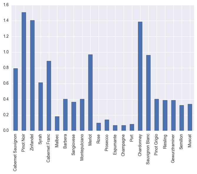
The most popular wines are Pinot Noir, Zinfandel, Merlot, Chardonnay, and Sauvignon Blanc.
Clustering:
X = data[data.columns]

# All column names (wine types) are stored as x_cols
x_cols = data.columns
I’ll use the elbow method to find the optimal number of clusters. This identifies the value of k (number of clusters) where the distortion (the within-cluster sum of squared errors or SSE) begins to increase the most rapidly.
distortions = []
for i in range (1,10):
    km = KMeans(n_clusters=i,
               init='k-means++',
               n_init=10,
               max_iter=300,
               random_state=0)
    km.fit(X)
    distortions.append(km.inertia_)

plt.plot(range(1,10), distortions, marker='o')
plt.xlabel('Number of clusters')
plt.ylabel('Distortion')
plt.show()
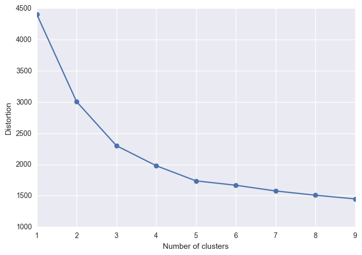
It looks like the elbow is located at k=3… We can also use the silhouette score; this is a measure of how similar an objects is to its own cluster compared to other clusters. The score is higher when clusters are dense and well separated. A score of 1 is the highest and a score of -1 is the lowest. Scores around zero indicate overlapping clusters.
silhouette = {}
for i in range (2,10):
    km = KMeans(n_clusters=i,
               init='k-means++',
               n_init=10,
               max_iter=300,
               tol=1e-04,
               random_state=0)
    km.fit(X)
    silhouette[i] = metrics.silhouette_score(X, km.labels_, metric='euclidean')

silhouette
{2: 0.31931332744051177,
 3: 0.36448555932200755,
 4: 0.31707194676835887,
 5: 0.32698272012743929,
 6: 0.31207073251298323,
 7: 0.26206479403635502,
 8: 0.26891906112067659,
 9: 0.24363780237120475}
k=3 gives the highest score, by a hair. In general these scores are not that high indicating that there will be a fair amount of overlap between clusters.
cluster3 = KMeans(n_clusters=3,
               init='k-means++',
               n_init=10,
               max_iter=300,
               tol=1e-04,
               random_state=0)
# Add a column that indicates which cluster each point falls into
data['cluster3'] = cluster3.fit_predict(X)

# Let's see how many are in each cluster
data.cluster3.value_counts()
0    155
1     77
2     56
Name: cluster3, dtype: int64
To visualize the data I will project the data to 2D.
pca = PCA(n_components=2)

data['x']=pca.fit_transform(data[x_cols])[:,0]
data['y']=pca.fit_transform(data[x_cols])[:,1]

clusters_2d = data[['cluster3', 'x', 'y']]
ggplot(clusters_2d, aes(x='x', y='y', color='cluster3')) + \
    scale_color_gradient(low='#E1FA72', high='#F46FEE') + \
    geom_point(size=75) + ggtitle("Customers Grouped by Cluster")
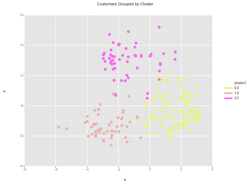
There is some overlap between the clusters. Let’s look at the clusters more closely and see what people are buying for each cluster.
Analyzing clusters:
# Making columns that indicate whether a customer is in a particular cluster
data['is_0'] = data.cluster3==0.0
data['is_1'] = data.cluster3==1.0
data['is_2'] = data.cluster3==2.0

just_wine = data.drop(['cluster3','x','y'],1)
# Let's group by cluster
cluster0 = just_wine.groupby('is_0').sum()
cluster1 = just_wine.groupby('is_1').sum()
cluster2 = just_wine.groupby('is_2').sum()
# Getting just the relevant row for each cluster
zero = cluster0.iloc[1:2]
one = cluster1.iloc[1:2]
two = cluster2.iloc[1:2]

# Let's put all the groups into one dataframe
all_clusters = zero.append(one, ignore_index=True)
all_clusters = all_clusters.append(two, ignore_index=True)
'''For some reason appending alphabetizes columns.
The previous ordering was more convenient because reds were with reds
and whites were with whites, so I'll go back to that column ordering.
'''
all_clusters = all_clusters.reindex_axis(cluster0.columns, axis=1)
all_clusters.drop(['is_1','is_2'], axis=1, inplace=True)
Now if you wanted to, you can see which wines are most/least popular for each cluster, and more easily look at differences between the clusters.
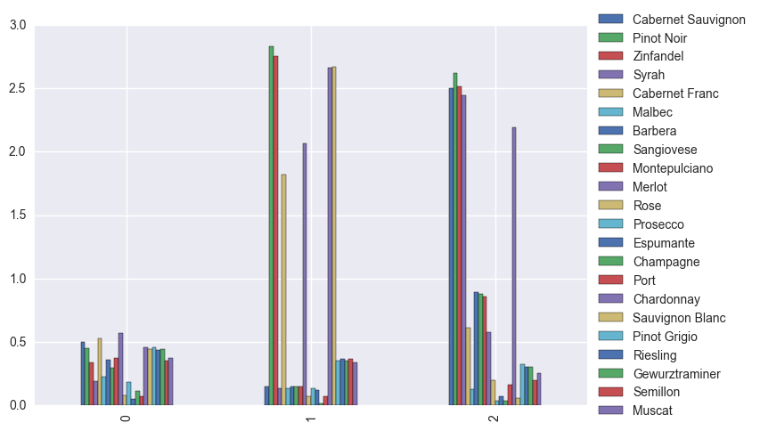
Most/least popular wines by cluster:
all_clusters.plot.bar().legend(loc='center left', bbox_to_anchor=(1, 0.5))
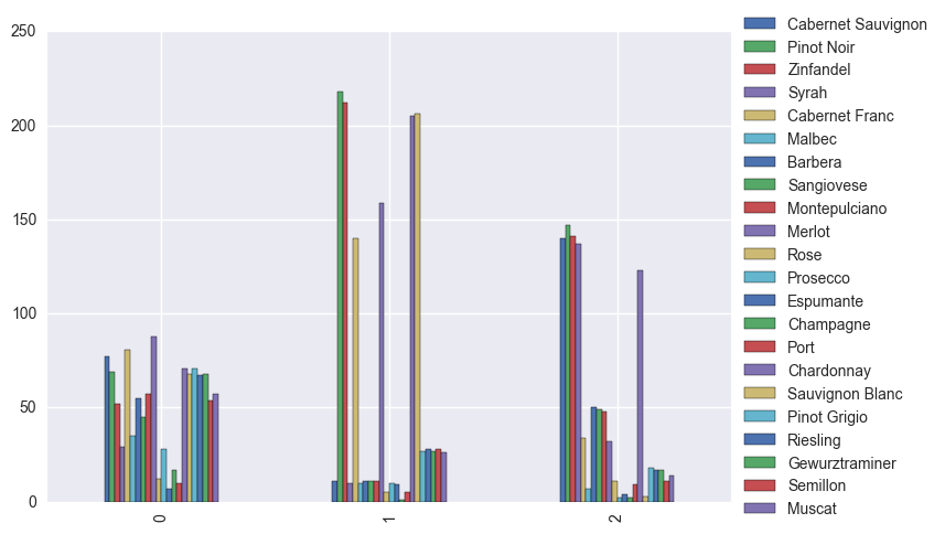
Just some observations: Most of the Pinot Noir, Zinfandel, Merlot, Chardonnay, and Sauvignon Blanc sales come from cluster 1. And most of the Syrah sales are coming from those in cluster 2.
I’m also interested in the mean purchases for each wine type, grouped by cluster.
cluster0_avg = just_wine.groupby('is_0').mean()
cluster1_avg = just_wine.groupby('is_1').mean()
cluster2_avg = just_wine.groupby('is_2').mean()
# Getting just the relevant row for each cluster
zero_avg = cluster0_avg.iloc[1:2]
one_avg = cluster1_avg.iloc[1:2]
two_avg = cluster2_avg.iloc[1:2]

# Let's put all the groups into one dataframe
all_clusters_avg = zero_avg.append(one_avg, ignore_index=True)
all_clusters_avg = all_clusters_avg.append(two_avg, ignore_index=True)
all_clusters_avg = all_clusters_avg.reindex_axis(zero_avg.columns, axis=1)
all_clusters_avg.drop(['is_1','is_2'], axis=1, inplace=True)
all_clusters_avg.plot.bar().legend(loc='center left', bbox_to_anchor=(1, 0.5))
Customers in cluster 0 buy less on average than the other two clusters, and don’t seem to have strong preferences when it comes to reds vs whites.
The customers in cluster 1 strongly prefer Pinot Noir, Zinfandel, Cabernet Franc, Merlot, Chardonnay, and Sauvignon Blanc over the other wines.
Customers in cluster 2 strongly prefer Cabernet Sauvignon, Pinot Noir, Zinfandel, Syrah, and Chardonnay, and buy more Italian wines on average.
Unsurprisingly, dessert or sparkling or special occasion wines (such as Prosecco, Espumante, Champagne) are low for all clusters.
Part 2- Building wine recommenders
In Part 1 I segmented customers based on the wines they bought. Here I’ll use the wine sales data to build wine recommenders.
from collections import defaultdict
import math
import numpy as np
from numpy import zeros, array, sqrt, log
import matplotlib.pyplot as plt
import scipy.sparse as sparse
from scipy.sparse.linalg import svds
from scipy.sparse import coo_matrix, csr_matrix, eye, diags, csc_matrix
from scipy.sparse.linalg import spsolve
import pandas as pd
import json
import operator
import time
Functions for calculating similarity: set or cosine based methods
def overlap(a,b):
    """
    Simple set based method to calculate similarity between two items.
    Looks at the number of users that the two items have in common.
    """
    return len(a.intersection(b))

def get_overlaps(item_sets, item_of_interest):
    """Get overlaps of multiple items with any item of interest"""
    for item in item_sets:
        print(item,':', overlap(item_sets[item_of_interest], item_sets[item]))

def norm2(v):
    """L2 norm"""
    return sqrt((v.data ** 2).sum())

def cosine(a, b):
    """Calculate the cosine of the angle between two vectors a and b"""
    return csr_matrix.dot(a, b.T)[0, 0] / (norm2(a) * norm2(b))

def get_sim_with_cos(items, item_of_interest):
    """Get overlaps of multiple items with any item of interest"""
    for item in items:
        print(item,':', cosine(items[item_of_interest], items[item]))
Functions for matrix factorization
def alternating_least_squares(Cui, factors, regularization=0.01,
                              iterations=15, use_native=True, num_threads=0,
                              dtype=np.float64):
    """
    Factorizes the matrix Cui using an implicit alternating least squares algorithm
    Args:
        Cui (csr_matrix): Confidence Matrix
        factors (int): Number of factors to extract
        regularization (double): Regularization parameter to use
        iterations (int): Number of alternating least squares iterations to
        run
        num_threads (int): Number of threads to run least squares iterations.
        0 means to use all CPU cores.
    Returns:
        tuple: A tuple of (row, col) factors
    """
    #_check_open_blas()

    users, items = Cui.shape

    X = np.random.rand(users, factors).astype(dtype) * 0.01
    Y = np.random.rand(items, factors).astype(dtype) * 0.01

    Cui, Ciu = Cui.tocsr(), Cui.T.tocsr()

    solver = least_squares

    for iteration in range(iterations):
        s = time.time()
        solver(Cui, X, Y, regularization, num_threads)
        solver(Ciu, Y, X, regularization, num_threads)
        print("finished iteration %i in %s" % (iteration, time.time() - s))

    return X, Y

def least_squares(Cui, X, Y, regularization, num_threads):
    """
    For each user in Cui, calculate factors Xu for them using least squares on Y.
    """
    users, factors = X.shape
    YtY = Y.T.dot(Y)

    for u in range(users):
        # accumulate YtCuY + regularization*I in A
        A = YtY + regularization * np.eye(factors)

        # accumulate YtCuPu in b
        b = np.zeros(factors)

        for i, confidence in nonzeros(Cui, u):
            factor = Y[i]
            A += (confidence - 1) * np.outer(factor, factor)
            b += confidence * factor

        # Xu = (YtCuY + regularization * I)^-1 (YtCuPu)
        X[u] = np.linalg.solve(A, b)

def bm25_weight(data, K1=100, B=0.8):
    """
    Weighs each row of the matrix data by BM25 weighting
    """
    # calculate idf per term (user)
    N = float(data.shape[0])
    idf = np.log(N / (1 + np.bincount(data.col)))

    # calculate length_norm per document
    row_sums = np.squeeze(np.asarray(data.sum(1)))
    average_length = row_sums.sum() / N
    length_norm = (1.0 - B) + B * row_sums / average_length

    # weight matrix rows by bm25
    ret = coo_matrix(data)
    ret.data = ret.data * (K1 + 1.0) / (K1 * length_norm[ret.row] + ret.data) * idf[ret.col]
    return ret

def nonzeros(m, row):
    """
    Returns the non zeroes of a row in csr_matrix
    """
    for index in range(m.indptr[row], m.indptr[row+1]):
        yield m.indices[index], m.data[index]
class ImplicitMF():
    '''
    Numerical value of implicit feedback indicates confidence that a user prefers an item.
    No negative feedback- entries must be positive.
    '''
    def __init__(self, counts, num_factors=40, num_iterations=30,
                 reg_param=0.8):
        self.counts = counts
        self.num_users = counts.shape[0]
        self.num_items = counts.shape[1]
        self.num_factors = num_factors
        self.num_iterations = num_iterations
        self.reg_param = reg_param

    def train_model(self):
        self.user_vectors = np.random.normal(size=(self.num_users,
                                                   self.num_factors))
        self.item_vectors = np.random.normal(size=(self.num_items,
                                                   self.num_factors))

        for i in range(self.num_iterations):
            t0 = time.time()
            print('Solving for user vectors...')
            self.user_vectors = self.iteration(True, csr_matrix(self.item_vectors))
            print('Solving for item vectors...')
            self.item_vectors = self.iteration(False, csr_matrix(self.user_vectors))
            t1 = time.time()
            print('iteration %i finished in %f seconds' % (i + 1, t1 - t0))

    def iteration(self, user, fixed_vecs):
        num_solve = self.num_users if user else self.num_items
        num_fixed = fixed_vecs.shape[0]
        YTY = fixed_vecs.T.dot(fixed_vecs)
        eye1 = eye(num_fixed)
        lambda_eye = self.reg_param * eye(self.num_factors)
        solve_vecs = np.zeros((num_solve, self.num_factors))

        t = time.time()
        for i in range(num_solve):
            if user:
                counts_i = self.counts[i].toarray()
            else:
                counts_i = self.counts[:, i].T.toarray()
            CuI = diags(counts_i, [0])
            pu = counts_i.copy()
            pu[np.where(pu != 0)] = 1.0
            YTCuIY = fixed_vecs.T.dot(CuI).dot(fixed_vecs)
            YTCupu = fixed_vecs.T.dot(CuI + eye1).dot(csr_matrix(pu).T)
            xu = spsolve(YTY + YTCuIY + lambda_eye, YTCupu)
            solve_vecs[i] = xu
            if i % 1000 == 0:
                print('Solved %i vecs in %d seconds' % (i, time.time() - t))
                t = time.time()

        return solve_vecs
Functions for getting recommendations
class TopRelated_useruser(object):
    def __init__(self, user_factors):
        # fully normalize user_factors, so can compare with only the dot product
        norms = np.linalg.norm(user_factors, axis=-1)
        self.factors = user_factors / norms[:, np.newaxis]

    def get_related(self, movieid, N=10):
        scores = self.factors.dot(self.factors[movieid]) # taking dot product
        best = np.argpartition(scores, -N)[-N:]
        return sorted(zip(best, scores[best]), key=lambda x: -x[1])

class TopRelated_itemitem(object):
    def __init__(self, movie_factors):
        # fully normalize movie_factors, so can compare with only the dot product
        norms = np.linalg.norm(movie_factors, axis=-1)
        self.factors = movie_factors / norms[:, np.newaxis]

    def get_related(self, movieid, N=10):
        scores = self.factors.T.dot(self.factors.T[movieid])
        best = np.argpartition(scores, -N)[-N:]
        return sorted(zip(best, scores[best]), key=lambda x: -x[1])

def print_top_items(itemname2itemid, recs):
    """Print recommendations and scores"""
    inv_dict = {v: k for k, v in itemname2itemid.items()}
    for item_code, score in recs:
        print(inv_dict[item_code], ":", score)
The data:
data = pd.read_csv('winedata.csv')
Normalize by the number of items bought and make each entry between 0 and 1.
data['bought_norm'] = data['bought'] / data.groupby('user')['bought'].transform(sum)
Simple set based method:
First I’ll use a very naive approach and calculate similarity between two items by looking at the number of users that the two items have in common.
# Create a dictionary of wine name to the set of their users
item_sets = dict((item, set(users)) for item, users in data.groupby('Item')['user'])
Out of curiosity I’ll look at Cabernet Sauvignon, which is one of the most popular wines.
get_overlaps(item_sets, 'Cabernet Sauvignon')
Malbec : 25
Champagne : 4
Rose : 14
Pinot Noir : 82
Port : 13
Espumante : 6
Montepulciano : 92
Muscat : 27
Cabernet Franc : 70
Semillon : 26
Cabernet Sauvignon : 111
Sangiovese : 87
Prosecco : 11
Gewurztraminer : 32
Barbera : 96
Chardonnay : 69
Syrah : 58
Zinfandel : 79
Pinot Grigio : 32
Merlot : 68
Riesling : 31
Sauvignon Blanc : 26
Cosine based method:
Define similarity by measuring the angle between each pair of items.
# map each username to a unique numeric value
userids = defaultdict(lambda: len(userids))
data['userid'] = data['user'].map(userids.__getitem__)

# map each item to a sparse vector of their users
items = dict((item, csr_matrix(
                (group['bought_norm'], (zeros(len(group)), group['userid'])),
                shape=[1, len(userids)]))
        for item, group in data.groupby('Item'))
get_sim_with_cos(items, 'Cabernet Sauvignon')
Malbec : 0.123625800145
Champagne : 0.00824398669704
Rose : 0.0507192514212
Pinot Noir : 0.347795969061
Port : 0.0703081275495
Espumante : 0.0227991298744
Montepulciano : 0.517771008213
Muscat : 0.0979917146104
Cabernet Franc : 0.257483140482
Semillon : 0.110152890452
Cabernet Sauvignon : 1.0
Sangiovese : 0.6970694479
Prosecco : 0.0358025433636
Gewurztraminer : 0.0798347122216
Barbera : 0.810335208496
Chardonnay : 0.293563364976
Syrah : 0.329877671582
Zinfandel : 0.340325942969
Pinot Grigio : 0.0794288775148
Merlot : 0.22765532905
Riesling : 0.110072665209
Sauvignon Blanc : 0.0426492580584
Matrix factorization methods:
Implicit matrix factorization and alternating least squares.
# Get a random sample from each user for the test data
test_data = data.groupby('user', as_index=False).apply(lambda x: x.loc[np.random.choice(x.index, 1, replace=False),:])

# Get the indices of the test data
l1 = [x[1] for x in test_data.index.tolist()]

# train data
train_data = data.drop(data.index[l1]).dropna()

train_data['user'] = train_data['user'].astype("category")
train_data['Item'] = train_data['Item'].astype("category")

print("Unique users: %s" % (len(train_data['user'].unique())))
print("Unique items: %s" % (len(train_data['Item'].unique())))
Unique users: 252
Unique items: 22
# create a sparse matrix.
buy_data = csc_matrix((train_data['bought_norm'].astype(float),
                   (train_data['Item'].cat.codes,
                    train_data['user'].cat.codes)))
# Dictionary for item: category code
itemid2itemname = dict(enumerate(train_data['Item'].cat.categories))
itemname2itemid = {v: k for k, v in itemid2itemname.items()}

# Dictionary for user: category code
userid2username = dict(enumerate(train_data['user'].cat.categories))
username2userid  = {v: k for k, v in userid2username.items()}
# Implicit MF
impl = ImplicitMF(buy_data.tocsr())
impl.train_model()

impl_ii = TopRelated_itemitem(impl.user_vectors.T)

# ALS
als_user_factors, als_item_factors = alternating_least_squares(bm25_weight(buy_data.tocoo()), 50)

als_ii = TopRelated_itemitem(als_user_factors.T)
Recommendations:
Now if you use the get_related method of either impl_ii or als_ii you can get recommendations. For example, looking at Cabernet Sauvignon again (category code 2):
itemname2itemid
{'Barbera': 0,
 'Cabernet Franc': 1,
 'Cabernet Sauvignon': 2,
 'Champagne': 3,
 'Chardonnay': 4,
 'Espumante': 5,
 'Gewurztraminer': 6,
 'Malbec': 7,
 'Merlot': 8,
 'Montepulciano': 9,
 'Muscat': 10,
 'Pinot Grigio': 11,
 'Pinot Noir': 12,
 'Port': 13,
 'Prosecco': 14,
 'Riesling': 15,
 'Rose': 16,
 'Sangiovese': 17,
 'Sauvignon Blanc': 18,
 'Semillon': 19,
 'Syrah': 20,
 'Zinfandel': 21}
Top 10 related items (IMF) sorted from high to low:
CabSauvRecs_impl = impl_ii.get_related(2)
CabSauvRecs_impl.sort(key=operator.itemgetter(1), reverse=True)
CabSauvRecs_impl

print_top_items(itemname2itemid, CabSauvRecs_impl)
Cabernet Sauvignon : 1.92640388658
Montepulciano : 0.982636897522
Barbera : 0.91181546732
Sangiovese : 0.801211866236
Pinot Noir : 0.493039509471
Merlot : 0.450261531423
Syrah : 0.430613949117
Cabernet Franc : 0.394405045211
Zinfandel : 0.349210924318
Chardonnay : 0.311731048352
The top 5 most related to Cabernet Sauvignon (aside from itself) are Montepulciano, Barbera, Sangiovese, Pinot Noir, Merlot. Note: this does not mean these wines are alike in terms of their properties since this is not a content based recommender (although this would be fun to build).
Top 10 related items (ALS) sorted from high to low:
CabSauvRecs_als = als_ii.get_related(2)
CabSauvRecs_als.sort(key=operator.itemgetter(1), reverse=True)

print_top_items(itemname2itemid, CabSauvRecs_als)
Cabernet Sauvignon : 1.98385577268
Barbera : 1.26980921153
Montepulciano : 1.23604203209
Pinot Noir : 1.23454763923
Sangiovese : 1.17589964622
Cabernet Franc : 0.887842151257
Chardonnay : 0.874804063605
Syrah : 0.828921865353
Zinfandel : 0.818015786071
Merlot : 0.803151198909
The top most related to Cabernet Sauvignon from ALS are similar (just in a slightly different order)
TO DO NEXT:
- Evaluation with the test data.
- Nice graphics including venn diagrams to show overlap of wines.
- Try out a content based recommender. With wines, I can imagine it would work well (a recommender based on various properties of the wines, such as fruitiness, alcohol content, or even chemical composition).