Predicting income brackets

Data: Income data from the UCI ML Repository
Techniques: Classification, random forest

Here I build quick models (using sklearn and H2O) to determine income bracket from imbalanced data- the income levels are binned at below 50k and above 50k.

Some of the features are:

Age
Marital Status
Income
Family Members
No. of Dependents
Tax Paid
Investment (Mutual Fund, Stock)
Return from Investments
Education
Spouse Education
Nationality
Occupation
Region in US
Race
Occupation category

from collections import defaultdict
from operator import itemgetter
import numpy as np
import pandas as pd
import sklearn as sk
from sklearn import metrics
from sklearn.model_selection import StratifiedShuffleSplit
from sklearn.preprocessing import StandardScaler, Imputer
from sklearn.model_selection import train_test_split, cross_val_score, GridSearchCV
from sklearn.metrics import roc_auc_score, confusion_matrix
from sklearn.ensemble import RandomForestClassifier
from h2o.estimators.random_forest import H2ORandomForestEstimator
from h2o.model.metrics_base import H2OBinomialModelMetrics
import h2o
import os
import sys
sys.path.append('../MLRecipes')

# machine learning helper code
import ml_helper as mlhelp

%matplotlib inline
import matplotlib.pyplot as plt
import matplotlib.font_manager
from matplotlib import rcParams
import seaborn as sns
sns.set_style("whitegrid")
sns.set_context("poster")

print('Python version: %s.%s.%s' % sys.version_info[:3])
print('numpy version:', np.__version__)
print('pandas version:', pd.__version__)
print('scikit-learn version:', sk.__version__)

Python version: 3.5.2
numpy version: 1.11.1
pandas version: 0.18.1
scikit-learn version: 0.18.1

# Preprocessing functions
def label_map(y):    
    """Encodes labels"""

    # For incomes above 50k
    if y == 50000:
        return 1
    elif y == '50000+.':
        return 1
    elif y == ' 50000+.':
        return 1

    # For incomes below 50k
    elif y == -50000:
        return 0
    elif y == '-50000':
        return 0

def isNan(num):
    """Test for Nan"""
    return num != num

def add_MDcol(df, col_list):
    """Add column for missing categorical data"""
    for col in col_list:
        df[col+'_missing'] = df[col].apply(isNan)

Data preprocessing

train = pd.read_csv('train.csv')
test = pd.read_csv('test.csv')

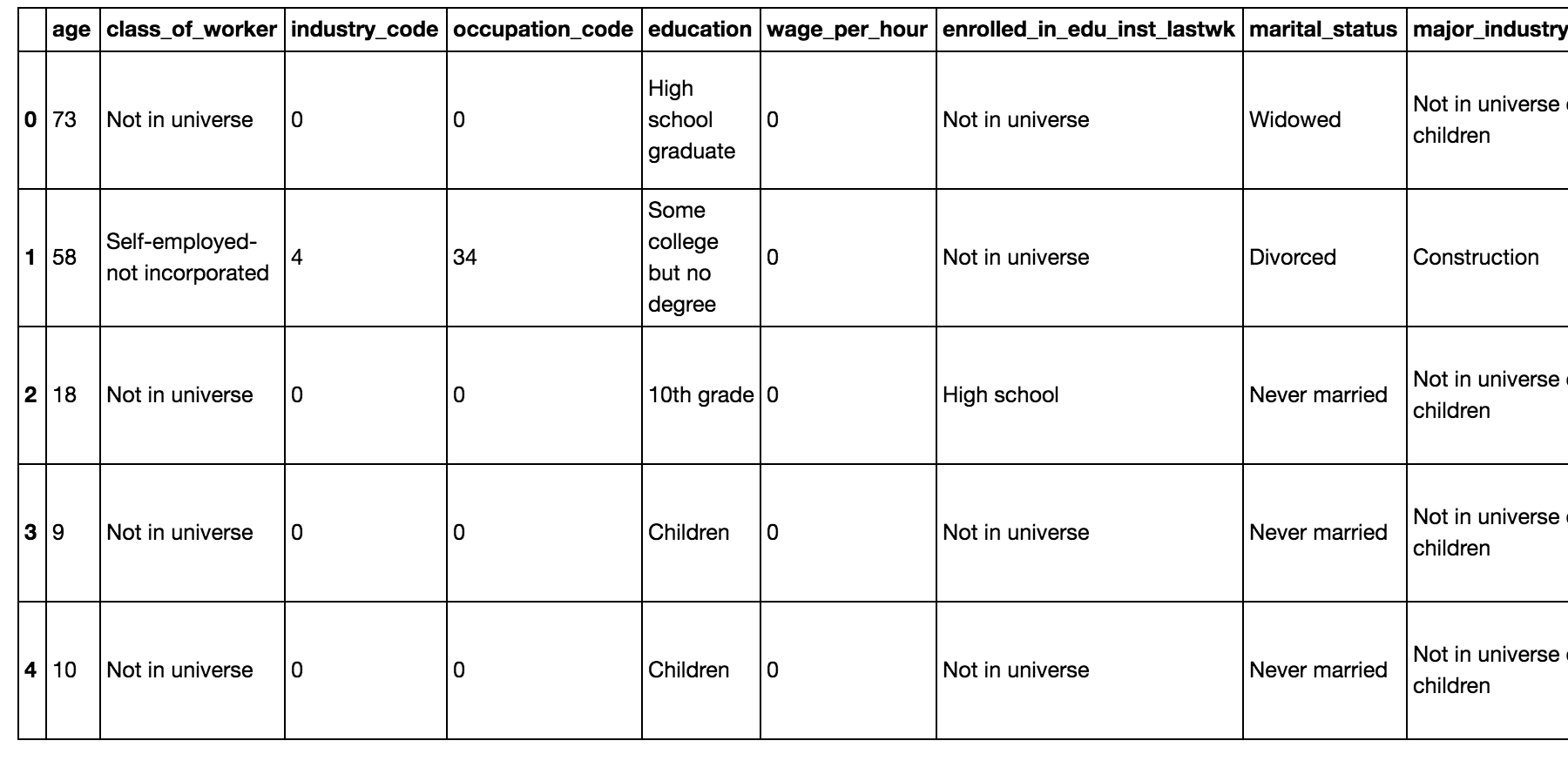
train.head()

png

train.shape

(199523, 41)

test.shape

(99762, 41)

The train data has 199,523 rows and 41 columns. The test data has 99,762 rows and 41 columns.

Cleanup

Let’s look at the labels:

train.income_level.value_counts()

-50000    187141
 50000     12382
Name: income_level, dtype: int64

test.income_level.value_counts()

-50000      93576
 50000+.     6186
Name: income_level, dtype: int64

Note: We have imbalanced classes here. The higher income class is about 6% of the total.

The labels are not written the same way. I’ll encode these variables as 0 and 1:

test['income_level'] = test['income_level'].apply(label_map)
train['income_level'] = train['income_level'].apply(label_map)

# Going to combine train and test from this dataset for now
alldata = train.append(test)

alldata.income_level.value_counts()

0    280717
1     18568
Name: income_level, dtype: int64

Check for missing values

alldata.isnull().values.any()

True

There are some missing values.

alldata.isnull().sum()

age                                     0
class_of_worker                         0
industry_code                           0
occupation_code                         0
education                               0
wage_per_hour                           0
enrolled_in_edu_inst_lastwk             0
marital_status                          0
major_industry_code                     0
major_occupation_code                   0
race                                    0
hispanic_origin                       874
sex                                     0
member_of_labor_union                   0
reason_for_unemployment                 0
full_parttime_employment_stat           0
capital_gains                           0
capital_losses                          0
dividend_from_Stocks                    0
tax_filer_status                        0
region_of_previous_residence            0
state_of_previous_residence           708
d_household_family_stat                 0
d_household_summary                     0
migration_msa                       99696
migration_reg                       99696
migration_within_reg                99696
live_1_year_ago                         0
migration_sunbelt                   99696
num_person_Worked_employer              0
family_members_under_18                 0
country_father                       6713
country_mother                       6119
country_self                         3393
citizenship                             0
business_or_self_employed               0
fill_questionnaire_veteran_admin        0
veterans_benefits                       0
weeks_worked_in_year                    0
year                                    0
income_level                            0
dtype: int64

All the missing values are part of categorical features. I’ll fill in the nans with “missing”- then when I do one-hot encoding this will essentially create an extra “missing” category.

Note: For H2O model implementations, we don’t have to fill in these nans, but we do for sklearn’s.

# Have to fill in nans for sklearn implementations
alldata_nonan = alldata.fillna(value='missing')

Explore data

sns.set(style='whitegrid',context='notebook')
cols=['age','wage_per_hour', 'capital_gains','capital_losses','dividend_from_Stocks' ,'d_household_family_stat','income_level']
sns.pairplot(alldata_nonan[cols],size=2.5)
plt.show()

png

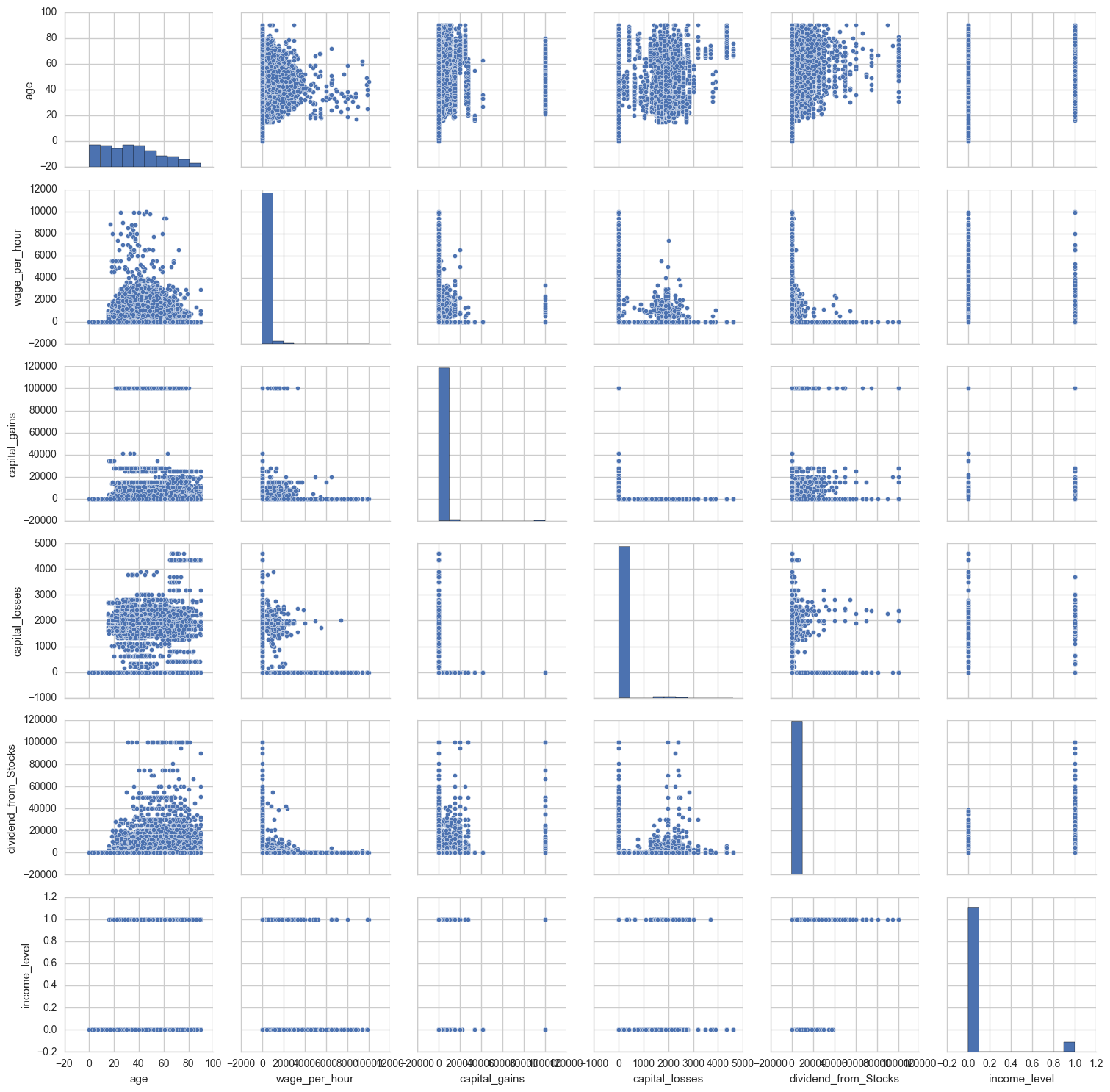
The lower income bracket has lower dividend_from_stocks. Unsurprisingly, none of the youngest people (under age 20) were in the higher income bracket. Interestingly wage_per_hour is not necessarily higher for the higher income bracket.

Quick random forest model

I’ll do a quick model for now before doing any feature engineering, etc.

col_list = list(alldata_nonan)
features = mlhelp.make_normal_features(alldata_nonan, col_list)

column_to_predict = 'income_level'

# Prepare data to be used in the model by transforming
# the lists of feature-value dictionaries to vectors
# When feature values are strings, the DictVectorizer will do a binary one-hot coding
X, y, dv, mabs = mlhelp.create_data_for_model(alldata_nonan, features, column_to_predict)

(X_train, X_test, y_train, y_test) = train_test_split(X, y, test_size=0.2,
                                                      stratify=y, random_state=2016)

rf = RandomForestClassifier(class_weight='balanced')
rf.fit(X_train, y_train)

y_predict = rf.predict(X_test)
mlhelp.classification_accuracy(y_truth=y_test, y_predict=y_predict);

Percentage correct predictions = 99.37
Percentage correct predictions (true class 0) = 99.99
Percentage correct predictions (true class 1) = 89.93

confmat = confusion_matrix(y_true=y_test, y_pred=y_predict)

fig,ax = plt.subplots(figsize=(2.5,2.5))
ax.matshow(confmat, cmap=plt.cm.Blues, alpha=0.3)
for i in range(confmat.shape[0]):
    for j in range(confmat.shape[1]):
        ax.text(x=j,y=i,
               s=confmat[i,j],
               va='center', ha='center')
plt.xlabel('predicted label')
plt.ylabel('true label')
plt.show()

png

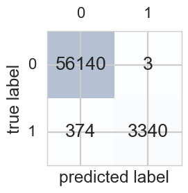
The classifier does a bit worse with class 1 (the rare class).
Some important features:

mlhelp.print_features_importances(rf, dv, max_print=10)

income_level 0.322192086021
num_person_Worked_employer 0.063498787871
occupation_code 0.0590363279715
weeks_worked_in_year 0.0523350224565
dividend_from_Stocks 0.0484704052559
age 0.0371623762101
industry_code 0.024954228483
major_occupation_code=Not in universe 0.022879498577
capital_gains 0.019464985337
family_members_under_18=Not in universe 0.0193774196446
tax_filer_status=Joint both under 65 0.0157218318548

Random forest (H2O)

The H2O implementation lets you work with categorical variables well (without one-hot encoding). You can also feed in missing values.

h2o.init(max_mem_size = "2G", nthreads=-1)

h2ofr = h2o.H2OFrame(alldata)

Parse progress: |█████████████████████████████████████████████████████████| 100%

h2ofr['income_level'] = h2ofr['income_level'].asfactor()

splits = h2ofr.split_frame(ratios=[0.7, 0.15], seed=1)
train = splits[0]
valid = splits[1]
test = splits[2]

y = 'income_level'
x = list(h2ofr.columns)

x.remove(y) # remove response variable

RF = H2ORandomForestEstimator(balance_classes=True)
RF.train(x=x, y=y, training_frame=train)

drf Model Build progress: |███████████████████████████████████████████████| 100%

RF_perf = RF.model_performance(test)
print(RF_perf)

ModelMetricsBinomial: drf
** Reported on test data. **

MSE: 0.03933510927017885
RMSE: 0.1983308076678428
LogLoss: 0.13454365044271357
Mean Per-Class Error: 0.12912999956069804
AUC: 0.9419047339083383
Gini: 0.8838094678166766
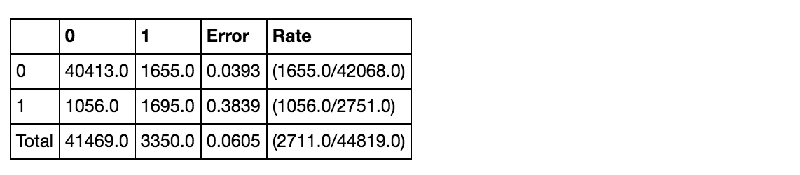
Confusion Matrix (Act/Pred) for max f1 @ threshold = 0.15341475654483194:

png

Maximum Metrics: Maximum metrics at their respective thresholds

png

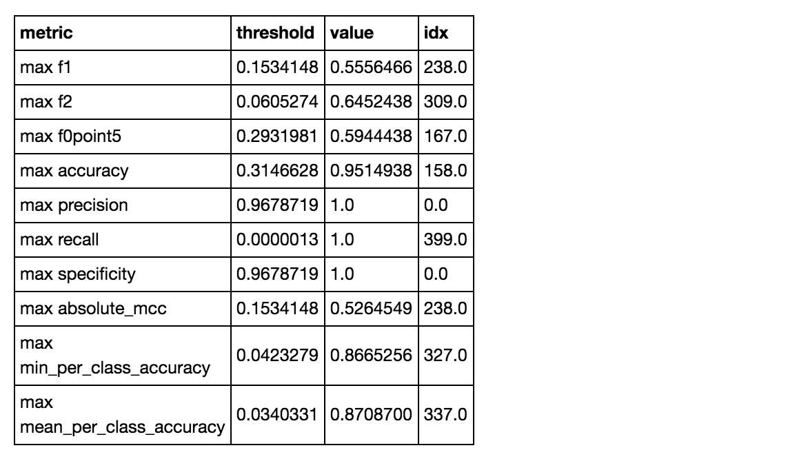
Gains/Lift Table: Avg response rate:  6.14 %

This one actually performs worse in predicting class 1 compared to the sklearn implementation. It only gets about 62% of class 1 right compared to getting 96% of class 0 right.