Explaining MCMC sampling

Data: Synthetic data
Techniques: MCMC

Metropolis Sampling

Code examples and annotations to explain the intuition behind the Metropolis sampling algorithm.

%matplotlib inline

import numpy as np
import scipy as sp
import pandas as pd
import matplotlib.pyplot as plt
import seaborn as sns
from scipy.stats import norm

sns.set_style('white')
sns.set_context('talk')

np.random.seed(123)

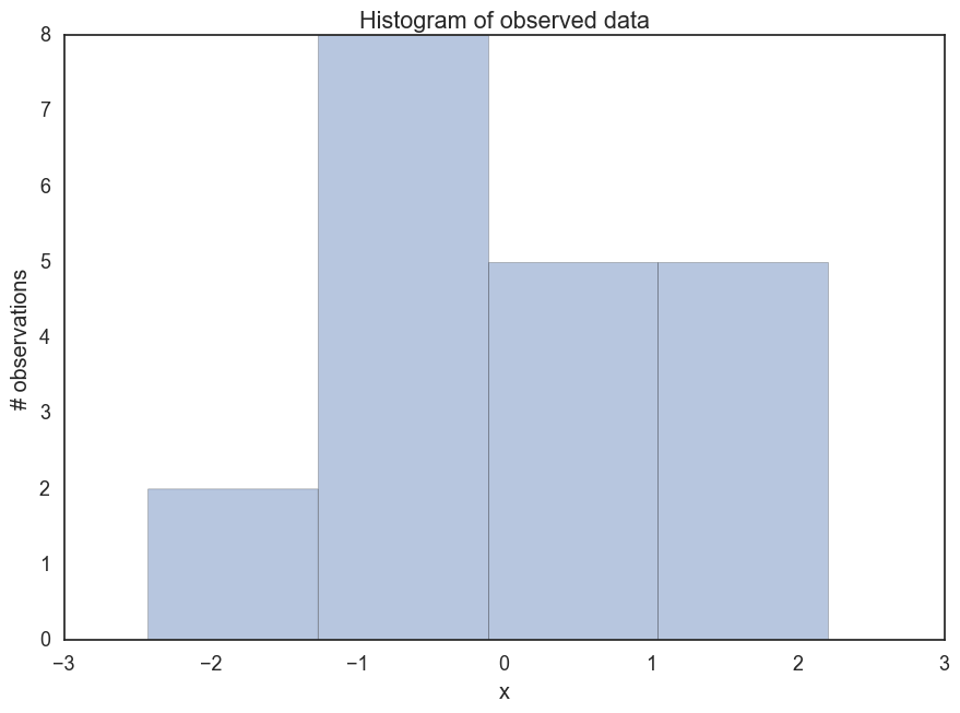
First let’s generate some made up data- 100 points from a standard normal distribution. Suppose we want to estimate the posterior of the mean mu. Of course for something simple like this, we wouldn’t need to use MCMC sampling. However, let’s forge ahead for illustration’s sake.

data = np.random.randn(20)

ax = plt.subplot()
sns.distplot(data, kde=False, ax=ax)
_ = ax.set(title='Histogram of observed data', xlabel='x', ylabel='# observations');

png

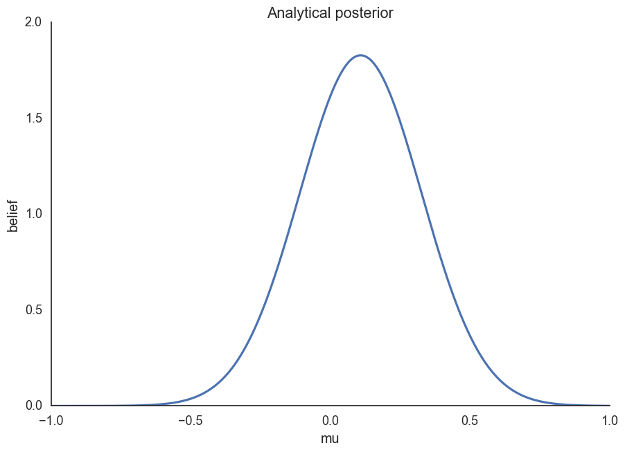
Let’s define our model. We will assume that this data is normally distributed. For simplicity we will assume we know that sigma = 1. For mu let’s assume a normal distribution as a prior. In this case we can compute the posterior analytically.

def calc_posterior_analytical(data, x, mu_0, sigma_0):
    sigma = 1.
    n = len(data)
    mu_post = (mu_0 / sigma_0**2 + data.sum() / sigma**2) / (1. / sigma_0**2 + n / sigma**2)
    sigma_post = (1. / sigma_0**2 + n / sigma**2)**-1
    return norm(mu_post, np.sqrt(sigma_post)).pdf(x)

ax = plt.subplot()
x = np.linspace(-1, 1, 500)
posterior_analytical = calc_posterior_analytical(data, x, 0., 1.)
ax.plot(x, posterior_analytical)
ax.set(xlabel='mu', ylabel='belief', title='Analytical posterior');
sns.despine()

png

How would we do this if we couldn’t solve this analytically?

Let’s see how we would do this if we couldn’t solve this by hand, and demonstrate how the Matropolis algorithm works.

At first you find a random starting parameter position. That’s mu_current.
Then you propose to move from that position to somewhere else. The Metropolis sampler just takes a sample from a “proposal distribution”- a normal distribution centered at your current mu value with a standard deviation (proposal_width) that determines how far you propose jumps (here we use scipy.stats.norm).
Next you evaluate whether to accept or reject the proposal- in other words, decide whether that’s a good place to jump or not. If the resulting normal distribution with that proposed_mu explains the data better than the old mu, you definitely go there. “Explains the data better” here means we compute the probability of the data, given the likelihood (normal) with the proposed parameter values (proposed mu and fixed sigma = 1).
We would just have a hill-climbing algorithm if this were all there was to the algorithm, so sometimes we have to accept moves in directions where the mu_proposal does not have higher likelihood than mu_current. The acceptance probability, p_accept, which is a ratio of p_proposal/p_current allows us to do just that. If p_proposal is larger than p_current, that ratio will be greater than 1 and we will accept. If p_current is larger, we will move with probability equal to p_accept.

def sampler(data, samples=4, mu_init=.5, proposal_width=.5, plot=False, mu_prior_mu=0, mu_prior_sd=1.):
    mu_current = mu_init
    posterior = [mu_current]
    
    for i in range(samples):
        
        # Propose to move from the initial position
        mu_proposal = norm(mu_current, proposal_width).rvs() # .rvs generates random samples
        
        # Compute likelihood by multiplying probabilities of each data point.
        # norm(mu,sd).pdf(n) gives the pdf values for data n, and prod.() takes their product
        likelihood_current = norm(mu_current, 1).pdf(data).prod() 
        likelihood_proposal = norm(mu_proposal, 1).pdf(data).prod()

        # Computer prior probability of current and proposed mu
        prior_current =  norm(mu_prior_mu, mu_prior_sd).pdf(mu_current)
        prior_proposal = norm(mu_prior_mu, mu_prior_sd).pdf(mu_proposal)

        # Nominator of Bayes formula
        p_current = likelihood_current * prior_current
        p_proposal = likelihood_proposal * prior_proposal
        
        # Accept proposal?
        p_accept = p_proposal / p_current
        
        # Usually would include prior probability, which we leave out for simplicity
        accept = np.random.randn() < p_accept
        
        if plot:
            plot_proposal(mu_current, mu_proposal, mu_prior_mu, mu_prior_sd, data, accept, posterior, i)
            
        if accept:
            mu_current = mu_proposal # update position 
            
        posterior.append(mu_current)
        
    return posterior

Why does this matter? Well we generally would be most interested in using MCMC for cases when we can’t compute P(data), aka the denominator in Bayes formula, or can’t approximate it using grid approximation (say, if we have many parameters and end up with a completely intractable integral). Since we are dividing posteriors here, the denominators cancel out nicely. This is how this procedure gives us samples from the posterior. In the end, we end up visiting regions of high posterior probability relatively more often that those of low posterior probability.

# Function to display
def plot_proposal(mu_current, mu_proposal, mu_prior_mu, mu_prior_sd, data, accepted, trace, i):
    from copy import copy
    trace = copy(trace)
    fig, (ax1, ax2, ax3, ax4) = plt.subplots(ncols=4, figsize=(16, 4))
    fig.suptitle('Iteration %i' % (i + 1))
    x = np.linspace(-3, 3, 5000)
    color = 'g' if accepted else 'r'
        
    # Plot prior
    prior_current = norm(mu_prior_mu, mu_prior_sd).pdf(mu_current)
    prior_proposal = norm(mu_prior_mu, mu_prior_sd).pdf(mu_proposal)
    prior = norm(mu_prior_mu, mu_prior_sd).pdf(x)
    ax1.plot(x, prior)
    ax1.plot([mu_current] * 2, [0, prior_current], marker='o', color='b')
    ax1.plot([mu_proposal] * 2, [0, prior_proposal], marker='o', color=color)
    ax1.annotate("", xy=(mu_proposal, 0.2), xytext=(mu_current, 0.2),
                 arrowprops=dict(arrowstyle="->", lw=2.))
    ax1.set(ylabel='Probability Density', title='current: prior(mu=%.2f) = %.2f\nproposal: prior(mu=%.2f) = %.2f' % (mu_current, prior_current, mu_proposal, prior_proposal))
    
    # Likelihood
    likelihood_current = norm(mu_current, 1).pdf(data).prod()
    likelihood_proposal = norm(mu_proposal, 1).pdf(data).prod()
    y = norm(loc=mu_proposal, scale=1).pdf(x)
    sns.distplot(data, kde=False, norm_hist=True, ax=ax2)
    ax2.plot(x, y, color=color)
    ax2.axvline(mu_current, color='b', linestyle='--', label='mu_current')
    ax2.axvline(mu_proposal, color=color, linestyle='--', label='mu_proposal')
    #ax2.title('Proposal {}'.format('accepted' if accepted else 'rejected'))
    ax2.annotate("", xy=(mu_proposal, 0.2), xytext=(mu_current, 0.2),
                 arrowprops=dict(arrowstyle="->", lw=2.))
    ax2.set(title='likelihood(mu=%.2f) = %.2f\nlikelihood(mu=%.2f) = %.2f' % (mu_current, 1e14*likelihood_current, mu_proposal, 1e14*likelihood_proposal))
    
    # Posterior
    posterior_analytical = calc_posterior_analytical(data, x, mu_prior_mu, mu_prior_sd)
    ax3.plot(x, posterior_analytical)
    posterior_current = calc_posterior_analytical(data, mu_current, mu_prior_mu, mu_prior_sd)
    posterior_proposal = calc_posterior_analytical(data, mu_proposal, mu_prior_mu, mu_prior_sd)
    ax3.plot([mu_current] * 2, [0, posterior_current], marker='o', color='b')
    ax3.plot([mu_proposal] * 2, [0, posterior_proposal], marker='o', color=color)
    ax3.annotate("", xy=(mu_proposal, 0.2), xytext=(mu_current, 0.2),
                 arrowprops=dict(arrowstyle="->", lw=2.))
    #x3.set(title=r'prior x likelihood $\propto$ posterior')
    ax3.set(title='posterior(mu=%.2f) = %.5f\nposterior(mu=%.2f) = %.5f' % (mu_current, posterior_current, mu_proposal, posterior_proposal))
    
    if accepted:
        trace.append(mu_proposal)
    else:
        trace.append(mu_current)
    ax4.plot(trace)
    ax4.set(xlabel='iteration', ylabel='mu', title='trace')
    plt.tight_layout()
    #plt.legend()

np.random.seed(123)
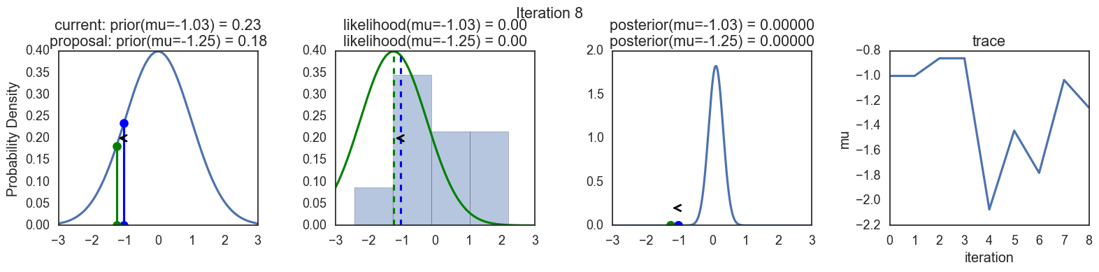
sampler(data, samples=8, mu_init=-1., plot=True);

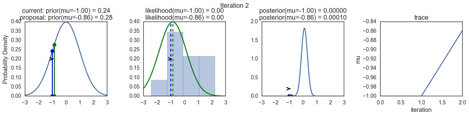
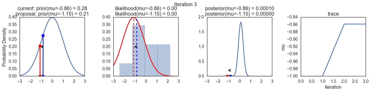
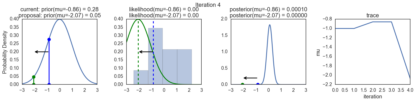
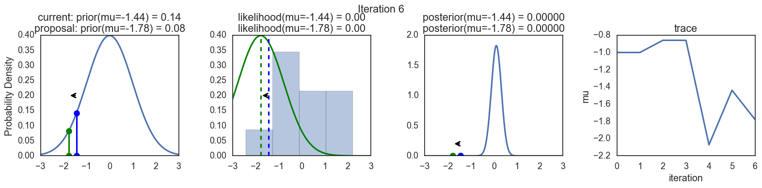
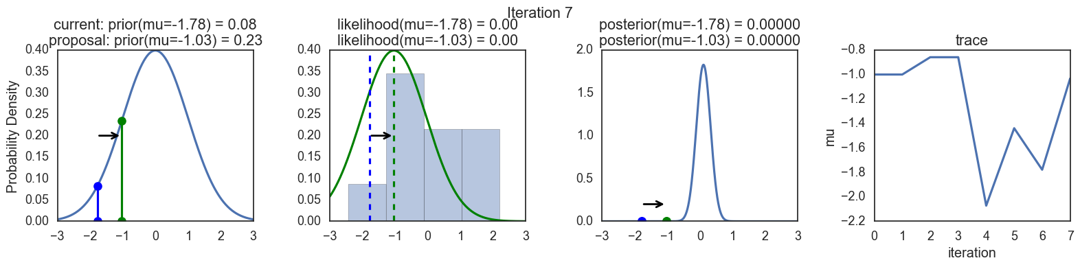
Finally, some plots to visualize the sampling. Each row is a single iteration through the Metropolis sampler. The columns are:

prior, 2. likelihood, 3. posterior, 4. trace (posterior samples of mu we are generating). The number of iteration is at the top center of each row.

png

Thanks to this post for more code and explanations.