
Sentiment analysis of political tweets
Data: Twitter API
Techniques: NLP, sentiment analysis with various models, scraping
Part 1- EDA and cleanup of tweets about Trump and Clinton
During the 2016 Presidential campaign, I collected a little over 270,000 tweets using the Twitter API and filtered for tweets that contained ‘Trump’, ‘DonaldTrump’, ‘Hillary’, ‘Clinton’, or ‘HillaryClinton’. The tweets were collected in July of 2016.
Twitter parameters: https://dev.twitter.com/streaming/overview/request-parameters#track
I’ll preprocess these tweets to do some exploratory analysis, look at the most common co-occurring words, and perform sentiment analysis.
Note: I did not have labeled data, so I used short movie reviews to train my model. This is not expected to lead to accurate predictions of sentiment in tweets (especially of ones that are political in nature), since this would not capture things like sarcasm (of which there is no shortage on Twitter). However, I did it anyway to try it out, and have a workflow ready for when I do have labeled data.
%matplotlib inline
import matplotlib.pyplot as plt
import seaborn as sns
from IPython.display import SVG
import json
import pandas as pd
import numpy as np
import re
from nltk.corpus import stopwords
import string
from collections import Counter
import operator
import sqlalchemy
import sqlite3 as sql
def add_column_for_name(df, names_list, text_column):
    """
    Add column(s) that indicates whether name(s) is/are in text_column
    Args:
        df: pandas dataframe
        names_list: list of strings (names)
        text_column: column containing text
    Returns:
        df with column of Booleans
    """
    for name in names_list:
        mydf[name] = mydf['text'].apply(lambda tweet: word_in_text(name, tweet))
    return df

def remove_retweets(df, column, list_of_str):
    """
    Function to remove tweets that contain string in list_of_str
    """
    for string in list_of_str:
        df = df[df['text'].str.contains(string)==False]
    return df

def print_val_counts_for_True(df, list_of_cols):
    """
    Print number of Trues for columns in list_of_cols in dataframe df
    """
    for name in list_of_cols:
        print(name, df[name].value_counts()[True])

def word_in_text(word, text):
    """
    Function to make text lower case and return True if a term is present, False otherwise
    """
    word = word.lower()
    text = text.lower()
    match = re.search(word, text)
    if match:
        return True
    return False

def lower_text(list_text):
    """
    Make text lowercase
    """
    new_list_text = []
    for word in list_text:
        new_word = word.lower()
        new_list_text.append(new_word)
    return new_list_text

def extract_link(text):
    """
    Extracting links from tweets
    """
    regex = r'https?://[^\s<>"]+|www\.[^\s<>"]+'
    match = re.search(regex, text)
    if match:
        return match.group()
    return ''

# Functions for tokenizing and preprocessing

def tokenize(s):
    return tokens_re.findall(s)

def preprocess(s, lowercase = False):
    tokens = tokenize(s)
    if lowercase:
        tokens = [token if emoticon_re.search(token) else token.lower() for token in tokens]
    return tokens

def tweet_tokenize(text):
    """
    Tokenize text
    """
    tweet_tokens = preprocess(text, lowercase = False)
    return tweet_tokens

def itertools_flatten(list_of_list):
    """
    Flatten out list of lists
    """
    from itertools import chain
    return list(chain(*list_of_list))

def most_frequent(terms_all, names_list):
    """
    Returns most frequent terms, aside from stop words. terms_all is a list with all the terms
    """
    count_all = Counter()
    full_stop = stop + names_list
    interesting_terms = [term for term in terms_all if term not in full_stop]

    # Update the counter
    count_all.update(interesting_terms)
    return count_all.most_common(20)

def make_col_lowercase(df, list_of_cols):
    """
    Function to get lowercase of columns in list_of_cols
    Args:
        df: pandas dataframe
        list_of_cols: list of column names (string)
    """
    for string in list_of_cols:
        df['lower_'+ string] = df[string].apply(lambda tweet: lower_text(tweet))
    return df
# Data is stored in an sqlite database. Reading sqlite query into a dataframe:
conn = sql.connect('tweets.db')
mydf = pd.read_sql_query('SELECT lang, text FROM lang_text', conn)
conn.close()

mydf.count()
lang    278713
text    278713
dtype: int64
mydf['text'].describe()
count     278713
unique    132656
top
freq       12012
Name: text, dtype: object
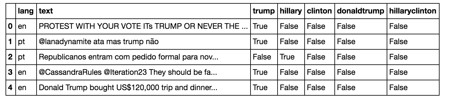
Adding columns that show whether the tweet contains a name of interest:
I decided to add columns of Booleans that indicated whether a name was in the tweet or not.
I’m also interested in weeding out tweets that might be about Bill Clinton.
Of course, while doing this I might be taking out tweets that are about the other kind of bill (legislative), but I’m going to assume that’s a negligible number.
# Add columns for names of interest
names_list = ['trump','hillary','clinton','donaldtrump','hillaryclinton','bill']
add_column_for_name(mydf, names_list ,'text')
# Count number of Trues for columns in list_of_cols
list_of_cols = ['trump', 'donaldtrump', 'hillary', 'clinton', 'hillaryclinton']
print_val_counts_for_True(mydf, list_of_cols)
trump 127268
donaldtrump 15999
hillary 94226
clinton 82198
hillaryclinton 23025
Some cleanup: removing retweets:
# Return df with duplicates removed. By default this keeps the first occurrence only.
unique_tweets = mydf.drop_duplicates(inplace=False, subset='text')

len(unique_tweets)
132656
# Remove retweets
list_of_str = ['RT', 'rt', ' RT ']
originals = remove_retweets(unique_tweets, 'text', list_of_str)
originals = originals.reset_index(drop = True)
originals.head()
len(originals)
95923
Counting names:
# Count number of Trues for columns in list_of_cols again, now with 'bill'
list_of_cols = ['trump', 'donaldtrump', 'hillary', 'clinton', 'hillaryclinton', 'bill']
print_val_counts_for_True(originals, list_of_cols)
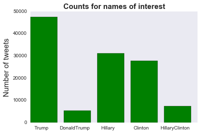
trump 47493
donaldtrump 5241
hillary 31054
clinton 27664
hillaryclinton 7391
bill 1453
Extract links:
originals['link'] = originals['text'].apply(extract_link)
Note: I added columns that indicated whether the tweet contained only one name and not the others (for example, just “clinton” and not “hillary” or “trump” or “bill”) as well as columns that indicated whether a name was present or not, regardless of whether other names were there.
# Getting value counts for names
list_of_cols = ['trump', 'donaldtrump', 'just_trump','hillary', 'clinton', 'hillaryclinton',
                'just_hillary','just_clinton','Any_Trump','Any_Clinton','Any_Clinton_no_bill']
print_val_counts_for_True(originals, list_of_cols)
trump 47493
donaldtrump 5241
just_trump 42252
hillary 31054
clinton 27664
hillaryclinton 7391
just_hillary 10727
just_clinton 8965
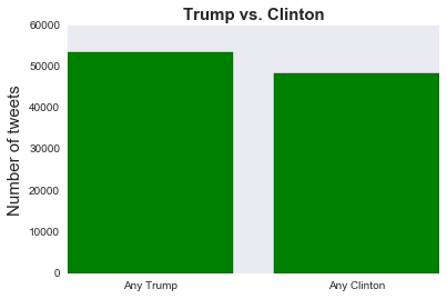
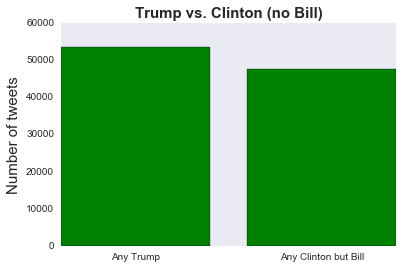
Any_Trump 53400
Any_Clinton 48430
Any_Clinton_no_bill 47394
A plot for counts for names of interest:
names = ['Trump', 'DonaldTrump', 'Hillary', 'Clinton', 'HillaryClinton']
tweets_by_name = [originals['trump'].value_counts()[True], originals['donaldtrump'].value_counts()[True], originals['hillary'].value_counts()[True], originals['clinton'].value_counts()[True], originals['hillaryclinton'].value_counts()[True]]
x_pos = list(range(len(names)))
width = 0.8
fig, ax = plt.subplots()
plt.bar(x_pos, tweets_by_name, width, alpha=1, color='g')
ax.set_ylabel('Number of tweets', fontsize=15)
ax.set_title('Counts for names of interest', fontsize=15, fontweight='bold')
ax.set_xticks([p + 0.4 * width for p in x_pos])
ax.set_xticklabels(names)
plt.grid()
plt.savefig('tweet_by_name_1', format='png')
# Term frequencies for any Trump tweets and any Hillary or Clinton tweets, but not ones that have both
names = ['Any Trump', 'Any Clinton']
tweets_by_name = [originals['Any_Trump'].value_counts()[True], originals['Any_Clinton'].value_counts()[True]]
x_pos = list(range(len(names)))
width = 0.8
fig, ax = plt.subplots()
plt.bar(x_pos, tweets_by_name, width, alpha=1, color='g')
ax.set_ylabel('Number of tweets', fontsize=15)
ax.set_title('Trump vs. Clinton', fontsize=15, fontweight='bold')
ax.set_xticks([p + 0.5 * width for p in x_pos])
ax.set_xticklabels(names)
plt.grid()
plt.savefig('tweet_by_name_1', format='png')
# Term frequencies for any Trump tweets and any Hillary or Clinton tweets, except the ones that contain 'Bill'
names = ['Any Trump', 'Any Clinton but Bill']
tweets_by_name = [originals['Any_Trump'].value_counts()[True], originals['Any_Clinton_no_bill'].value_counts()[True]]
x_pos = list(range(len(names)))
width = 0.8
fig, ax = plt.subplots()
plt.bar(x_pos, tweets_by_name, width, alpha=1, color='g')
ax.set_ylabel('Number of tweets', fontsize=15)
ax.set_title('Trump vs. Clinton (no Bill)', fontsize=15, fontweight='bold')
ax.set_xticks([p + 0.5 * width for p in x_pos])
ax.set_xticklabels(names)
plt.grid()
plt.savefig('tweet_by_name_1', format='png')
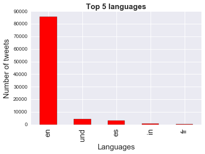
Languages:
# Tweets by language
tweets_by_lang = originals['lang'].value_counts() #get the counts for the lang column
fig, ax = plt.subplots()
ax.tick_params(axis = 'x', labelsize=15)
ax.tick_params(axis = 'y', labelsize=10)
ax.set_xlabel('Languages', fontsize=15)
ax.set_ylabel('Number of tweets' , fontsize=15)
ax.set_title('Top 5 languages', fontsize=15, fontweight='bold')
tweets_by_lang[:5].plot(ax=ax, kind='bar', color='red')
Pre-processing tweets:
# For pre-processing emoticons, @-mentions, hash-tags, URLs

emoticons_str = r"""
    (?:
        [:=;] # Eyes
        [oO\-]? # Nose (optional)
        [D\)\]\(\]/\\OpP] # Mouth
    )"""

regex_str = [
    emoticons_str,
    r'<[^>]+>', # HTML tags
    r'(?:@[\w_]+)', # @-mentions
    r"(?:\#+[\w_]+[\w\'_\-]*[\w_]+)", # hash-tags
    r'http[s]?://(?:[a-z]|[0-9]|[$-_@.&+]|[!*\(\),]|(?:%[0-9a-f][0-9a-f]))+', # URLs

    r'(?:(?:\d+,?)+(?:\.?\d+)?)', # numbers
    r"(?:[a-z][a-z'\-_]+[a-z])", # words with - and '
    r'(?:[\w_]+)', # other words
    r'(?:\S)' # anything else
]

# re.compile compiles a regex pattern into a regex object that can be used for match or search

tokens_re = re.compile(r'('+'|'.join(regex_str)+')', re.VERBOSE | re.IGNORECASE)
emoticon_re = re.compile(r'^'+emoticons_str+'$', re.VERBOSE | re.IGNORECASE)

# Add column of tokenized tweets
originals['tweet_tokens'] = originals['text'].apply(lambda tweet: tweet_tokenize(tweet))
Adding columns for tokens:
originals['tweet_tokens'].head()
0    [PROTEST, WITH, YOUR, VOTE, ITs, TRUMP, OR, NE...
1                [@lanadynamite, ata, mas, trump, não]
2    [Republicanos, entram, com, pedido, formal, pa...
3    [@CassandraRules, @Iteration23, They, should, ...
4    [Donald, Trump, bought, US, $, 120,000, trip, ...
Name: tweet_tokens, dtype: object
# Adding a column for the tokens and also selecting for just the English ones
originals['just_trump_tokens'] = np.where((originals['lang']== 'en') & (originals['Any_Trump'] ==True), originals['tweet_tokens'], '')
originals['just_clinton_tokens'] = np.where((originals['lang']== 'en') & (originals['Any_Clinton_no_bill'] ==True), originals['tweet_tokens'], '')
eng_trump_tokens = originals['just_trump_tokens'].values.tolist()
eng_clinton_tokens = originals['just_clinton_tokens'].values.tolist()

trump_list = itertools_flatten(eng_trump_tokens)
clinton_list = itertools_flatten(eng_clinton_tokens)

trump_list = [x.lower() for x in trump_list]
clinton_list = [x.lower() for x in clinton_list]
list_of_cols = ['tweet_tokens', 'just_trump_tokens', 'just_clinton_tokens']
originals = make_col_lowercase(originals, list_of_cols)
Getting ready to count most frequent words by getting rid of stopwords, punctuation:
# string.punctuation gives string of ASCI chars which are considered punctuation chars
punctuation = list(string.punctuation)
more_punctuation = ["’", "‘"]

# A custom list of stopwords
more_stops = ["el", "don't", "it's", "get", "via", "rt", "de", "would", "make",
            "i'm", "2", "he's", "one", "says","amp", "say", "us", "u"]

# The full stop list contains English stopwords, as well as my custom list of stopwords and punctuation to remove
stop = stopwords.words('english') + punctuation + more_punctuation + more_stops

trump_names_list = ['trump', 'donald', 'donaldtrump', '#trump', '@realdonaldtrump', "trump's"]
clinton_names_list= ['clinton', 'hillary', 'hillaryclinton', '@hillaryclinton']
Most frequent words associated with both candidates:
Words that co-occurred most frequently with Clinton

Words that co-occurred most frequently with Trump.

Part 2- Sentiment Analysis of Tweets about Trump and Clinton
Now I’ll perform sentiment analysis of the tweets.
%matplotlib inline
import seaborn as sns
import matplotlib.pyplot as plt
import plotly.plotly as py
import plotly.tools as tls
from ggplot import *

import pandas as pd
import numpy as np
import nltk
from nltk import word_tokenize
from sklearn.model_selection import train_test_split
from nltk.classify.scikitlearn import SklearnClassifier
from sklearn.naive_bayes import MultinomialNB, BernoulliNB
from sklearn.linear_model import LogisticRegression
from sklearn.svm import LinearSVC
import sys
sys.path.append('../MLRecipes')
import ml_helper as mlhelp
import pickle
import random
def find_features(words):
    """Takes as input a list of tokenized words and outputs features"""
    features = {}
    for w in word_features:
        features[w] = (w in words) # the dict has the word as key and boolean as value
    return features

def classify_list(classifier, token_list):
    """Get predicted label from classifier"""
    values = []
    for nested_list in token_list:
        value = classifier.classify(find_features(nested_list))
        values.append(value)
    return values
Training and testing:
Note: I did not have labeled tweets for this project, but I did find a collection of short movie reviews that had been labeled as negative or positive. I will use these to train my model; this is far from perfect since tweets are probably really different from short movie reviews, but it’s better than nothing.
# The short positive and negative review samples
short_pos = open("short_reviews_from_pyprognet/positive.txt","r").read()
short_neg = open("short_reviews_from_pyprognet/negative.txt","r").read()
# Prep the reviews
documents = []

for r in short_pos.split('\n'):
    documents.append( (r, "pos") )
for r in short_neg.split('\n'):
    documents.append( (r, "neg") )

all_words = []
short_pos_words = word_tokenize(short_pos)
short_neg_words = word_tokenize(short_neg)

for w in short_pos_words:
    all_words.append(w.lower())
for w in short_neg_words:
    all_words.append(w.lower())

# This will be the words and their frequencies
all_words = nltk.FreqDist(all_words)

# Get the first 5000 words from all_words
word_features = list(all_words.keys())[:5000]

# Save the feature existence booleans and their respective pos or neg categories. Example: (words, pos) -> ({words: True}, pos)
featuresets = [(find_features(rev), category) for (rev, category) in documents]

# Shuffle in place:
random.shuffle(featuresets)

# This data set has ~10600+ features
training_set = featuresets[:10000]
testing_set = featuresets[10000:]
Testing a few algorithms:
Trying a few different implementations of Naive Bayes.
classifier = nltk.NaiveBayesClassifier.train(training_set)

MNB_classifier = SklearnClassifier(MultinomialNB())
MNB_classifier.train(training_set)

BNB_classifier = SklearnClassifier(BernoulliNB())
BNB_classifier.train(training_set)
I’ll also try logistic regression and SVM.
LR_classifier = SklearnClassifier(LinearSVC())
LR_classifier.train(training_set)

SVM_classifier = SklearnClassifier(LogisticRegression())
SVM_classifier.train(training_set)
The accuracies were similar for the different models:
NLTK Naive Bayes algorithm accuracy percent:  67.37160120845923
Multinomial Naive Bayes accuracy percent: 68.42900302114803
Bernoulli Naive Bayes accuracy percent: 67.97583081570997
Logistic Regression accuracy percent: 65.25679758308158
SVM accuracy percent: 67.97583081570997
Most informative features:
A glance at which words were most informative:
classifier.show_most_informative_features(15)
Most Informative Features
               wonderful = True              pos : neg    =     18.0 : 1.0
                intimate = True              pos : neg    =     15.5 : 1.0
                   guise = True              neg : pos    =     12.5 : 1.0
              heartbreak = True              pos : neg    =     11.5 : 1.0
                provides = True              pos : neg    =     11.3 : 1.0
                   inept = True              neg : pos    =     11.1 : 1.0
                mindless = True              neg : pos    =     11.1 : 1.0
                   banal = True              neg : pos    =     11.1 : 1.0
                   knock = True              neg : pos    =     10.4 : 1.0
                   flaws = True              pos : neg    =      9.3 : 1.0
                  flawed = True              pos : neg    =      9.3 : 1.0
              meandering = True              neg : pos    =      9.1 : 1.0
                 iranian = True              pos : neg    =      8.9 : 1.0
                touching = True              pos : neg    =      8.5 : 1.0
                   mixed = True              neg : pos    =      8.4 : 1.0
Tweets about Trump:
multiple_bars=plt.figure()
x=['MultNaiveBayes', 'BernNaiveBayes', 'LogisticReg', 'SVM']
ind=np.arange(len(x))
pos = all_trump_pos
neg = all_trump_neg

ax.set_title("Trump's Positive and Negative Tweets")
ax=plt.subplot(111)
ax.bar(ind-.2, pos, width=.2, color='g', align='center', label='Pos')
ax.bar(ind, neg, width=.2, color='r', align='center', label='Neg')

ax.set_xticks(ind)
ax.set_xticklabels(x)
ax.set_ylabel('Number of Tweets')
ax.set_xlabel('Model')
ax.legend(loc='best')
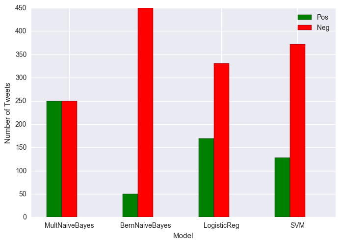
Percent negative MNB classifier: 50.0
Percent negative BNB classifier: 90.0
Percent negative LR classifier: 66.2
Percent negative SVM classifier: 74.4
Red is negative and green is positive.
Tweets about Clinton:
multiple_bars=plt.figure()
x=['MultNaiveBayes', 'BernNaiveBayes', 'LogisticReg', 'SVM']
ind=np.arange(len(x))
pos = all_clinton_pos
neg = all_clinton_neg

ax.set_title("Clinton's Positive and Negative Tweets")
ax=plt.subplot(111)
ax.bar(ind-.2, pos, width=.2, color='g', align='center', label='Pos')
ax.bar(ind, neg, width=.2, color='r', align='center', label='Neg')

ax.set_xticks(ind)
ax.set_xticklabels(x)
ax.set_ylabel('Number of Tweets')
ax.set_xlabel('Model')
ax.legend(loc='best')
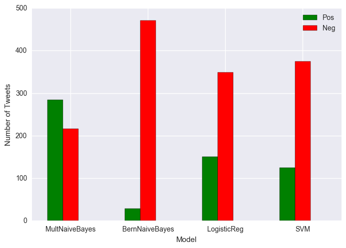
Percent negative MNB classifier: 43.2
Percent negative BNB classifier: 94.19999999999999
Percent negative LR classifier: 69.8
Percent negative SVM classifier: 75.0
Red is negative and green is positive.
The tweets were mostly classified as negative for both candidates. Of course these classifiers are not great for tweets, because they were trained on short movie reviews. In particular I’m guessing that movie reviews don’t use as many acronyms as tweets. And I can also imagine that they’re generally less sarcastic than tweets.
If I were to try to improve on the classifier I’d get some tweets labeled, and also include more classes so that in addition to “positive” and “negative” I’d have “neutral” and maybe also “sarcastic.” I’d also explore whether emoticons were predictive of sentiment.