
Predicting non-functional water pumps in Tanzania
Data: Competition for drivendata.org
Techniques: Classification, random forest, PCA
Part I- EDA and cleanup
Part II- Model selection and evaluation
Part I- EDA and cleanup
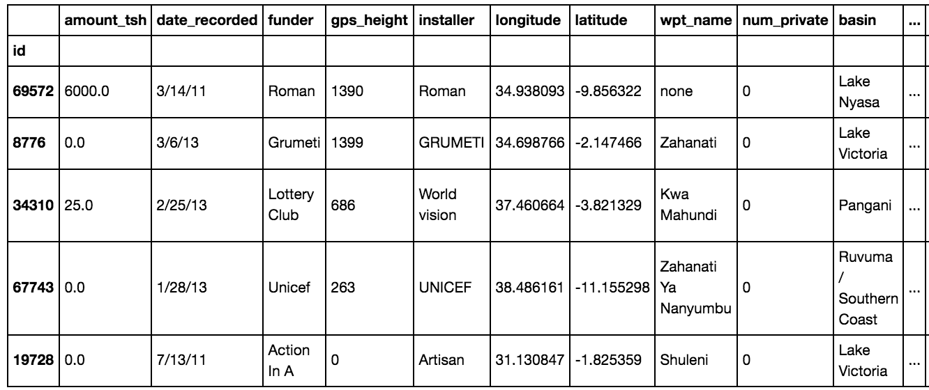
Using data on water pumps in communities across Tanzania, can we predict the pumps that are functional, need repairs, or don’t work at all?
There are 39 features in total. They are described here.
%matplotlib inline
import matplotlib.pyplot as plt
from matplotlib.pylab import rcParams
import seaborn as sns
import pandas as pd
import numpy as np
import sys

import sklearn as sk
from sklearn import metrics
from sklearn.model_selection import train_test_split, ShuffleSplit, learning_curve, GridSearchCV
from sklearn.preprocessing import StandardScaler, Imputer
from sklearn.feature_selection import SelectKBest
from sklearn.pipeline import Pipeline
from sklearn.metrics import classification_report, confusion_matrix
from sklearn.ensemble import RandomForestClassifier, GradientBoostingClassifier
from sklearn.linear_model import LogisticRegression
from sklearn.svm import SVC

print('Python version: %s.%s.%s' % sys.version_info[:3])
print('numpy version:', np.__version__)
print('pandas version:', pd.__version__)
print('scikit-learn version:', sk.__version__)
Python version: 3.5.2
numpy version: 1.12.0
pandas version: 0.19.2
scikit-learn version: 0.18.1
def label_map(y):
    """
    Converts string labels to integers
    """
    if y=="functional":
        return 2
    elif y=="functional needs repair":
        return 1
    else:
        return 0


def isNan(num):
    """
    Function to test for Nan. Returns True for NaNs, False otherwise.
    """
    return num != num
# Load the data
train = pd.read_csv('training.csv', index_col='id')
labels = pd.read_csv('train_labels.csv', index_col='id')
test = pd.read_csv('test_set.csv', index_col='id')
train.head()
print("Train data labels:",len(labels))
print("Train data rows, columns:",train.shape)
print("Test data rows, columns:", test.shape)
Train data labels: 59400
Train data rows, columns: (59400, 39)
Test data rows, columns: (14850, 39)
Visualizing water pumps:
Apparently responsibility for water and sanitation service provision is decentralized, so local governments are responsible for water resource management. Luckily, we have information on which regions the water pumps are in. Perhaps this will be a good predictor.
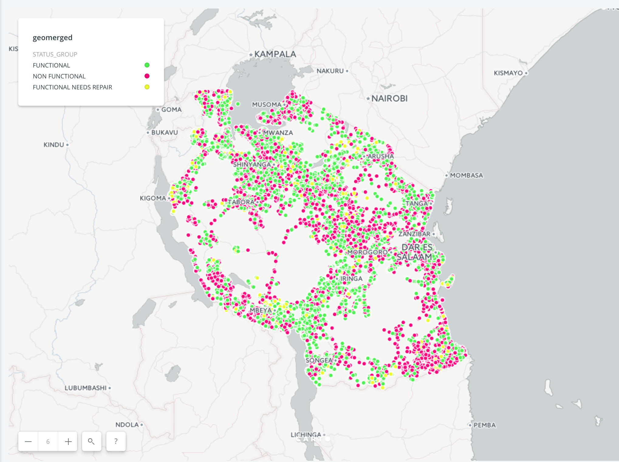
There is some “clumpiness” here; in the southeast you’ll notice that there seems to be a higher proportion of non-functional pumps (red) than near Iringa, where you see a lot of green (functional).
Exploring the data:
# Pairwise plots
sns.set(style='whitegrid',context='notebook')
cols=['amount_tsh','gps_height','num_private','population','status_group']
sns.pairplot(merged[cols],size=2.5)
plt.show()
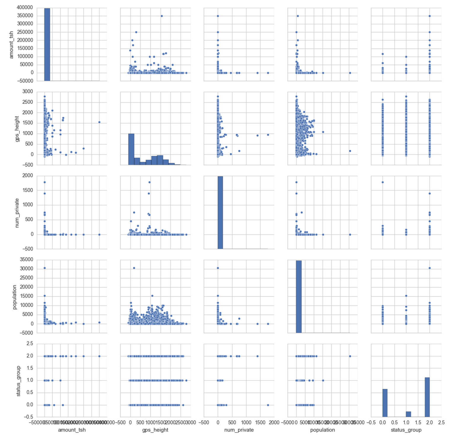 The variables plotted here are:
- amount_tsh: total static head (amount water available to waterpoint)
- gps_height: altitude of well
- num_private: (this feature is not described)
- population: population around the well
It looks like the water pumps with high static head tend to be functional (label 2). (It would also be worth looking into whether the really high tsh values are realistic.)
Funders:
Apparently water resource management in Tanzania relies heavily on external donors (according to my rudimentary research). We have 1898 different funders in this dataset, with a lot of missing values. There are also many funders with too few observations to have any real impact on model fit (many funders that only occur once).
len(train.funder.value_counts(dropna=False))
1898
train.funder.value_counts(dropna=False)
Government Of Tanzania            9084
NaN                               3636
Danida                            3114
Hesawa                            2202
Rwssp                             1374
World Bank                        1349
Kkkt                              1287
World Vision                      1246
Unicef                            1057
Tasaf                              877
District Council                   843
Dhv                                829
Private Individual                 826
Dwsp                               811
0                                  776
Norad                              765
Germany Republi                    610
Tcrs                               602
Ministry Of Water                  590
Water                              583
Dwe                                484
Netherlands                        470
Hifab                              450
Adb                                448
Lga                                442
Amref                              425
Fini Water                         393
Oxfam                              359
Wateraid                           333
Rc Church                          321
                                  ...
Alia                                 1
Kamata Project                       1
Mbozi Hospital                       1
Ballo                                1
Natherland                           1
Pankrasi                             1
Mzee Mkungata                        1
Cocu                                 1
H4ccp                                1
Redekop Digloria                     1
Luke Samaras Ltd                     1
John Gileth                          1
Samwel                               1
St Elizabeth Majengo                 1
Serikaru                             1
Municipal Council                    1
Dae Yeol And Chae Lynn               1
Rotary Club Kitchener                1
Camartec                             1
Chuo                                 1
Okutu Village Community              1
Kipo Potry                           1
Dmd                                  1
Maswi Drilling Co. Ltd               1
Lee Kang Pyung's Family              1
Grazie Grouppo Padre Fiorentin       1
Rudep /dwe                           1
Artisan                              1
Afriican Reli                        1
Makondakonde Water Population        1
Name: funder, dtype: int64
In addition to the 3635 NaNs, there are 777 that have the entry “0”.
I’m assuming these are missing values too, so altogether we have 4412 missing values.
Some other problems with this data:
A summary of other things to deal with in this dataset:
- installer: has NaNs, zeros, and many low frequency levels
- scheme_name: has NaNs and many low frequency levels
- scheme_management has NaNs
- population: has zeros and many low frequency levels*
- construction_year: has zeros
- permit: has NaNs
- public_meeting: has NaNs
Some options for dealing with this missing data:
- Drop the rows (I don’t want to do this in this case because this would be a large proportion of the data).**
- Mean/median/mode imputation (crude, can severely distort the distribution of the variable).
- Predict (in order to do this, features need to be correlated or related somehow).
- Create new feature like “no funder data.”
- For the missing categorical variables, I’m going to use option 4.
- For the missing population, I’ll leave the zeros as is, for the first pass at building a model, but at some point later on I might try to predict these using (for example) clustering or knn.
- For the missing construction_year, I’ll add a ‘missing_construction_year’ feature, and also run my model with and without imputation with the median. In a later iteration, maybe I’ll try to impute using a fancier algorithmn.
* Note on population:
If I were really thorough I would try to fill in missing population data using some kind of census data. Also I looked into using the (previously dropped) subvillage feature here to predict missing population values, but it does not seem like a good idea, because it appears that the population they report here (presumably some small radius around the water pump) is not just the subvillage population. That is, when I looked at population values for subvillages, entries with the same subvillage often had wildly different populations.
** Note on missing values:
It’s easy to imagine here that some of these NaNs may not be missing at random (we can imagine that year info is missing more from older wells, for example).
# Prep- convert the zeros in 'funder','installer', and 'population' to NaNs.
merged_clean = merged.replace({'funder':0, 'installer':0, 'population':0}, np.nan)
merged_clean = merged.replace({'funder':'0', 'installer':'0'}, np.nan)
Dealing with low frequency/many levels:
For these cases I will take low frequency levels (those that occur 20 times or less) and set to “other.” The 20 here is totally arbitrary; in the interest of time I won’t test out different thresholds or ways to bin, but ideally I would use cross validation to try out different methods and look at the effect on model performance.
# Lump low frequency levels in funder, installer, scheme_name into 'other'
exempt=['amount_tsh',  'gps_height',  'num_private',
       'basin', 'region', 'region_code', 'district_code', 'lga', 'population',
       'public_meeting', 'scheme_management',  'permit',
       'construction_year', 'extraction_type', 'extraction_type_group',
       'extraction_type_class', 'management', 'management_group', 'payment',
       'payment_type', 'water_quality', 'quality_group', 'quantity',
       'quantity_group', 'source', 'source_type', 'source_class',
       'waterpoint_type', 'waterpoint_type_group']

merged_clean = merged_clean.apply(lambda x: x.mask(x.map(x.value_counts())<20, 'other') if x.name not in exempt else x)
Construction year:
Replace zeros with NaNs. It might also be a good idea to bin the construction_year feature, but I will leave it as it is for this first pass.
merged_clean = merged.replace({'construction_year':0}, np.nan)
merged_clean = merged.replace({'construction_year':'0'}, np.nan)
# Note: this changed year values to floats
merged_clean.construction_year.value_counts(dropna=False)
NaN        20709
 2010.0     2645
 2008.0     2613
 2009.0     2533
 2000.0     2091
 2007.0     1587
 2006.0     1471
 2003.0     1286
 2011.0     1256
 2004.0     1123
 2012.0     1084
 2002.0     1075
 1978.0     1037
 1995.0     1014
 2005.0     1011
 1999.0      979
 1998.0      966
 1990.0      954
 1985.0      945
 1980.0      811
 1996.0      811
 1984.0      779
 1982.0      744
 1994.0      738
 1972.0      708
 1974.0      676
 1997.0      644
 1992.0      640
 1993.0      608
 2001.0      540
 1988.0      521
 1983.0      488
 1975.0      437
 1986.0      434
 1976.0      414
 1970.0      411
 1991.0      324
 1989.0      316
 1987.0      302
 1981.0      238
 1977.0      202
 1979.0      192
 1973.0      184
 2013.0      176
 1971.0      145
 1960.0      102
 1967.0       88
 1963.0       85
 1968.0       77
 1969.0       59
 1964.0       40
 1962.0       30
 1961.0       21
 1965.0       19
 1966.0       17
Name: construction_year, dtype: int64
Adding feature for missing construction year data:
merged_clean['missing_construction_year'] = merged_clean['construction_year'].apply(lambda x: isNan(x))
Summary of the number of missing values for each column:
merged_clean.isnull().sum()
amount_tsh                       0
funder                        3636
gps_height                       0
installer                     3656
num_private                      0
basin                            0
region                           0
region_code                      0
district_code                    0
lga                              0
population                       0
public_meeting                3334
scheme_management             3877
scheme_name                  28166
permit                        3056
construction_year            20709
extraction_type                  0
extraction_type_group            0
extraction_type_class            0
management                       0
management_group                 0
payment                          0
payment_type                     0
water_quality                    0
quality_group                    0
quantity                         0
quantity_group                   0
source                           0
source_type                      0
source_class                     0
waterpoint_type                  0
waterpoint_type_group            0
status_group                     0
missing_construction_year        0
dtype: int64
Interesting to note that the number of NaNs for both the funder and installer columns is close. If we compare just these two columns we see that the NaNs often appear in the same rows:
pd.concat([merged_clean.funder, merged_clean.installer], axis=1)
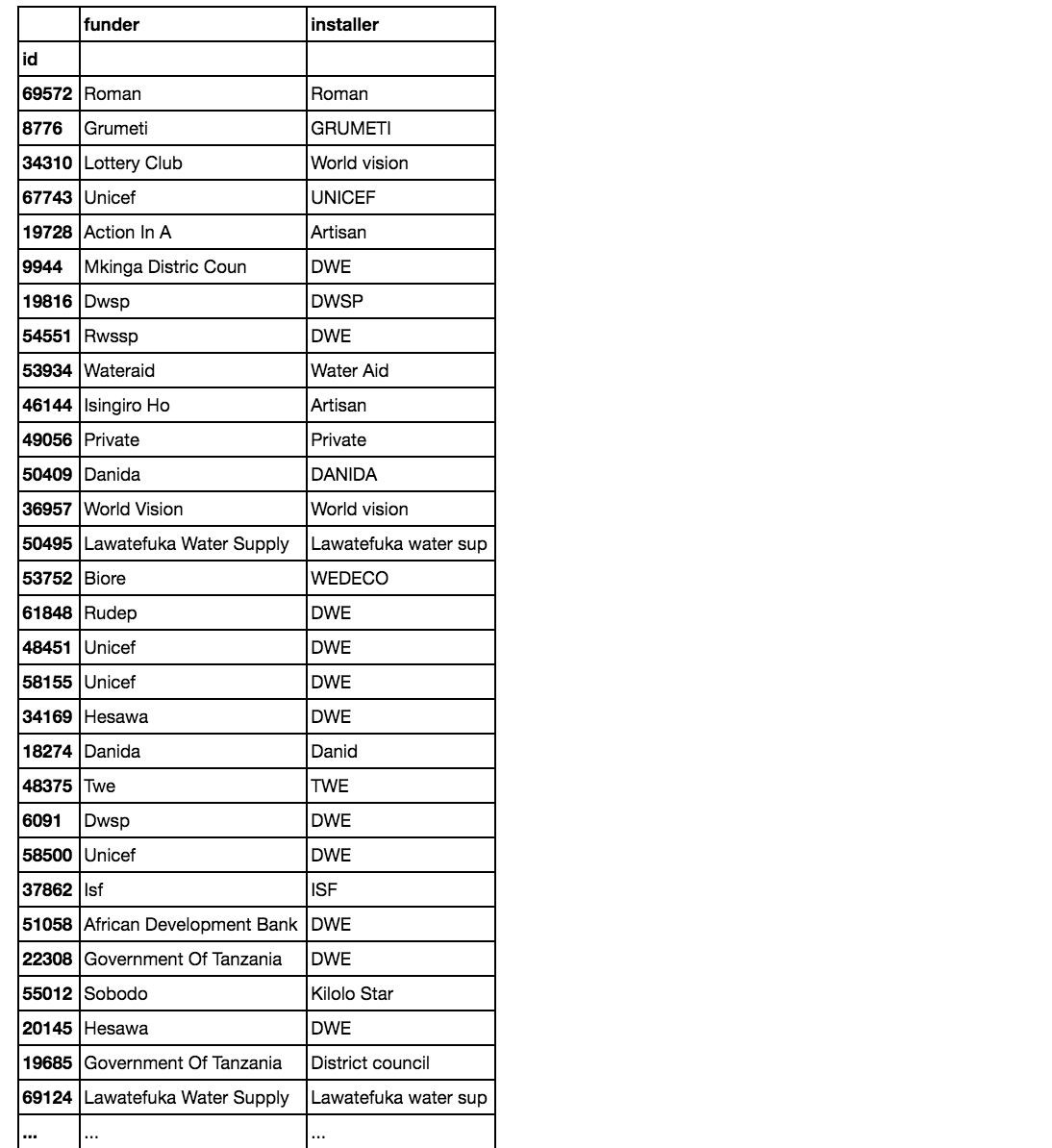
Something to notice here: the funder and installer is often the same entitiy.
When they are not the same, it’s usually because ‘DWE’ appears as the installer. It seems like ‘DWE’ could be some code for something (like “no information”), instead of an actual installer. Anyway, I will leave these alone in the absence of more information on what the acronyms mean.
Also there are some cases where the same entitiy was probably entered differently- for example “Danida” and “Danid” or “Jaica” and “JAICA CO” or “Government of Tanzania” and “Government” or “Wateraid” and “Water Aid” I won’t try to fix these for now, but this is something one would do ideally.
Dealing with categorical variables:
Convert categorical variables into dummy/indicator variables. At the same time, we’ll be adding columns to indicate NaNs.
merged_clean_dum = pd.get_dummies(merged_clean, dummy_na=True)
merged_clean_dum.shape
(59400, 7069)
I now have 7069 features.
merged_clean_dum.to_csv('merged_clean_dum.csv')
A note on other features of interest for this project:
It’s easy to imagine that we could improve our predictions with other sources of data here. Some that come to mind in this case are:
- Presence of other utilities nearby
- Rate of previous breakdowns
- Distance to major road
- Whether the water pump is in a hazardous or flooding area
- Crime rate in the near vicinity
Part II - Model selection and evaluation
I will try modeling two ways: (1) on one-hot encoded data, with and without dimensionality reduction, and (2) on the original data without one-hot encoding.
# Load the one-hot encoded data
data = pd.read_csv('merged_clean_dum.csv', index_col='id')
print("Data rows, columns:", data.shape)
Data rows, columns: (59400, 7069)
Note: region_code and district_code are integers, but categorical. I could convert these to dummy variables too, but I will leave these as is for the first pass.
# Getting just the features by dropping the labels
train = data.drop('status_group',1)

# Getting labels
labels = data.status_group
Model preprocessing and selection:
X = train.as_matrix()
y = labels.tolist()

X_train, X_test, y_train, y_test = \
    train_test_split(X, y, test_size=0.3, random_state=0)
I. GridSearchCV w/the one-hot encoded data:
Imputation, dimensionality reduction, and selection of hyperparameters for a random forest classifier (Note- I’m not testing hyperparameters exhaustively for now):
imputer = Imputer(strategy='median')
pca = decomposition.PCA()
rf = RandomForestClassifier(class_weight='balanced',
                            n_jobs=-1,
                            n_estimators=300)

steps = [('imputer', imputer),
        ('pca', pca),
        ('random_forest', rf)]

pipeline = Pipeline(steps)
parameters = dict(
                pca__n_components=[40, 100, 300],
                random_forest__max_features=['auto', 'log2']
                )

gs = GridSearchCV(pipeline, param_grid=parameters)
gs.fit(X_train, y_train)
print(gs.best_score_)
print(gs.best_params_)
0.773400673401
{'random_forest__max_features': 'log2', 'pca__n_components': 100}
Here are the best parameters.
rf = gs.best_estimator_
rf.fit(X_train, y_train)

y_pred = rf.predict(X_test)
print(classification_report(y_test, y_pred))
             precision    recall  f1-score   support

          0       0.82      0.76      0.79      6875
          1       0.41      0.39      0.40      1333
          2       0.80      0.85      0.82      9612

avg / total       0.78      0.78      0.78     17820
Classification report:
The model has an f1-score of about 0.8 for labels 0 and 2 (non-functional and functional), but does poorly on label 1.
Steps:
- Median imputation
- PCA with n_components=100
- Random Forest w/max_features=log2
(Note: I could refine hyperparameters further but I’ll move ahead for now).
rf.steps
[('imputer',
  Imputer(axis=0, copy=True, missing_values='NaN', strategy='median', verbose=0)),
 ('pca',
  PCA(copy=True, iterated_power='auto', n_components=100, random_state=None,
    svd_solver='auto', tol=0.0, whiten=False)),
 ('random_forest',
  RandomForestClassifier(bootstrap=True, class_weight='balanced',
              criterion='gini', max_depth=None, max_features='log2',
              max_leaf_nodes=None, min_impurity_split=1e-07,
              min_samples_leaf=1, min_samples_split=2,
              min_weight_fraction_leaf=0.0, n_estimators=300, n_jobs=-1,
              oob_score=False, random_state=None, verbose=0,
              warm_start=False))]
rf.steps[2][1]
RandomForestClassifier(bootstrap=True, class_weight='balanced',
            criterion='gini', max_depth=None, max_features='log2',
            max_leaf_nodes=None, min_impurity_split=1e-07,
            min_samples_leaf=1, min_samples_split=2,
            min_weight_fraction_leaf=0.0, n_estimators=300, n_jobs=-1,
            oob_score=False, random_state=None, verbose=0,
            warm_start=False)
importances = rf.steps[2][1].feature_importances_
std = np.std([tree.feature_importances_ for tree in rf.steps[2][1].estimators_],
             axis=0)
indices = np.argsort(importances)[::-1]
feature_names = np.array(list(train.columns.values))
feature_names
array(['amount_tsh', 'gps_height', 'num_private', ...,
       'waterpoint_type_group_improved spring',
       'waterpoint_type_group_other', 'waterpoint_type_group_nan'],
      dtype='<U58')
important_names = feature_names[importances>np.mean(importances)]
print(important_names)
['amount_tsh' 'gps_height' 'region_code' 'district_code' 'population'
 'construction_year' 'missing_construction_year' 'funder_0'
 'funder_A/co Germany' 'funder_Aar' 'funder_Abas Ka' 'funder_Abasia'
 'funder_Abc-ihushi Development Cent' 'funder_Abd' 'funder_Abdala'
 'funder_Abood' 'funder_Abs' 'funder_Aco/germany' 'funder_Acord Ngo'
 'funder_Act' 'funder_Act Mara' 'funder_Africa Project Ev Germany'
 'funder_Africaone Ltd' 'funder_Aqua Blues Angels' 'funder_Area']
Top features:
Some of the top features are: amount_tsh (total static head, or amount water available to waterpoint), gps_height (altitude of the well), region and district codes, population, construction year, missing construction year, and funder.
Some caveats:
This is not unique to using random forests for feature selection, but applies to most model based feature selection methods: if the dataset has correlated features, once one of them is used as a predictor, the importance of the others is significantly reduced. This is ok if we just want to use feature selection to avoid overfitting, but if we are using it to interpret the data, we have to be careful.
Problems with one-hot encoding:
When we one-hot encoded categorical variables, the resulting sparsity makes continuous variables assigned higher feature importance. Moreover, a single level of a categorical variable must meet a very high bar to be selected for splitting early in the tree building, which can degrade predictive performance. Lastly, by one-hot encoding, we created many binary variables, and they were all seen as independent (from the splitting algorithm’s point of view).
Confusion matrix:
confmat = confusion_matrix(y_true=y_test, y_pred=y_pred)
confmat
array([[5216,  217, 1442],
       [ 211,  523,  599],
       [ 911,  539, 8162]])
fig,ax = plt.subplots(figsize=(2.5,2.5))
ax.matshow(confmat, cmap=plt.cm.Blues, alpha=0.3)
for i in range(confmat.shape[0]):
    for j in range(confmat.shape[1]):
        ax.text(x=j,y=i,
               s=confmat[i,j],
               va='center', ha='center')
plt.xlabel('predicted label')
plt.ylabel('true label')
plt.show()
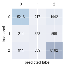
The model has the most trouble classifying water pumps in class 1 (pumps that need repair).
II. H2O implementation of random forest without one-hot encoding:
The H2O random forest implementation lets you input categorical data without one-hot encoding. It also treats missing values differently than sklearn’s (as a separate category).
Start up a local H2O cluster:
h2o.init(max_mem_size = "2G", nthreads=-1)
Import data:
This is a cleaned up version of the data without one-hot encoding.
data2 = h2o.import_file(os.path.realpath('merged_clean.csv'))
Parse progress: |█████████████████████████████████████████████████████████| 100%
Encode response variable:
Since we want to train a classification mode, we must ensure that the response is coded as a factor.
data2['status_group']=data2['status_group'].asfactor() # encode response as a factor
data2['status_group'].levels() # show the levels
[['0', '1', '2']]
Partition data:
# Partition data into 70%, 15%, 15% chunks
# Setting a seed will guarantee reproducibility
train, valid, test = data2.split_frame([0.7, 0.15], seed=1234)
X = data2.col_names[1:-1] # All columns except first (id) and last (reponse variable)
y = data2.col_names[-1] # Response variable
Model:
I’ll quickly build a model for now and come back to tuning hyperparameters later.
rf_v1 = H2ORandomForestEstimator(
        model_id="rf_v1",
        balance_classes=True,
        ntrees=300,
        stopping_rounds=2,
        score_each_iteration=True,
        seed=1000000)
rf_v1.train(X, y, training_frame=train, validation_frame=valid)
drf Model Build progress: |███████████████████████████████████████████████| 100%
rf_v1
Model Details
=============
H2ORandomForestEstimator : Distributed Random Forest
Model Key: rf_v1
Model Summary:
ModelMetricsMultinomial: drf
** Reported on train data. **
MSE: 0.24663297395089073
RMSE: 0.496621560094697
LogLoss: 0.7351344533214206
Mean Per-Class Error: 0.34878276470320757
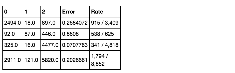
Confusion Matrix: vertical: actual; across: predicted
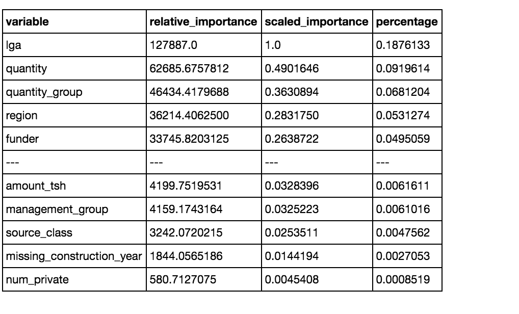
Variable Importances:
Just like in the sklearn implementation, from looking at the confusion marix we can see that the error is highest with label 1. It does relatively well with labels 0 and 2.
The top features are also different from what we saw with the sklearn implementation, which upweighted the importance of continuous variables. In the H2O implementation the top features are all categorical.